Reliability Growth Analysis and Plots

[Please note that the following article — while it has been updated from our newsletter archives — may not reflect the latest software interface and plot graphics, but the original methodology and analysis steps remain applicable.]

Portrait of Beautiful Caucasian Woman Working on Laptop Computer at a Bright Creative Office. Young Female Manager Updating Employees' Schedules and Answering Colleagues' E.mails

During the first phases of a product's development, the estimate of the product's final reliability is called the reliability goal. However, the first prototypes produced will almost certainly contain design, manufacturing and/or engineering deficiencies that prevent the product from reaching that goal. In order to identify and correct these deficiencies, prototypes are usually subjected to a rigorous testing program and appropriate corrective actions are implemented to improve the design. This structured process of finding reliability problems and monitoring the increase of the product's reliability through successive phases is called reliability growth.

Until now, the software available for analyzing reliability growth data has been fairly limited. However, ReliaSoft is currently working in cooperation with Dr. Larry Crow, the premier expert in the field of reliability growth, to develop the next generation of reliability growth analysis software, RGA. This article presents a brief overview of the capabilities of RGA and an introduction to some of the results and plots that are available for your reliability growth and related analyses.

RGA 6 Overview

The RGA software includes a wide variety of features to aid you in your reliability growth analyses so that you not only can obtain the results, but also understand the results. Features include:

Data entry spreadsheets support continuous (time-to-failure), discrete (success/failure) and reliability data.
Data analysis with the major reliability growth models: Crow (AMSAA), Gompertz, Modified Gompertz, Logistic and Lloyd-Lipow. Maximum Likelihood Estimation (MLE) is used for parameter estimation.
Projections analysis using A, B and C failure mode classifications and the definition of effectiveness factors for use in the Crow (AMSAA) Projection model. This model can be used to estimate the number of unseen failure modes, the maximum achievable reliability and other important metrics.
Repairable systems (overhauls) analysis using the Crow (AMSAA) model and Dr. Crow's analysis methodology.
Chi-Squared and CVM methods for goodness-of-fit testing (depending on the data type) as well as the Statistical Test for Growth.
Expanded plotting capabilities and automated custom reports created in Microsoft Word and Excel.
The ability to attach any type of file to the analysis. For example, you can attach an Excel file that has the original data or a Word document that contains the report based on the data analysis.

Basic Analysis Results and Plots

Although the results and plots that can be generated for your analysis will depend on the type of data that you have collected and the reliability growth model selected for analysis, some basic plots and results can be generated for all analyses. Figures 1 and 2 demonstrate two plots that present reliability growth results over time. Figure 1 presents the expected number of failures and Figure 2 presents the instantaneous MTBF.

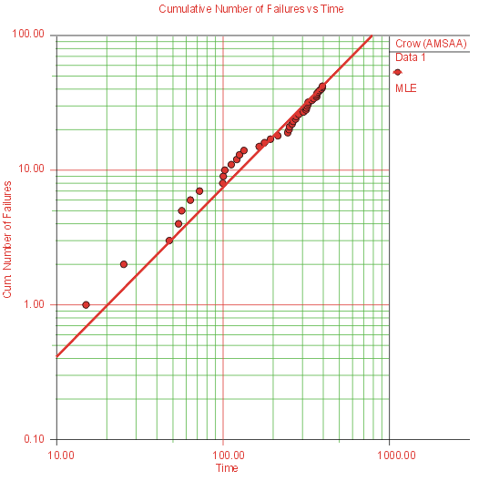
Figure 1: Expected Number of Failures vs. Time

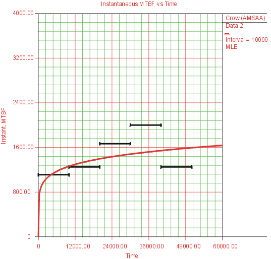
Figure 2: Instantaneous MTBF vs. Time

RGA’s QCP also provides point estimates for these metrics given time. In addition, you can generate charts and results for the cumulative MTBF and similar output for instantaneous and cumulative failure rates.

Reliability Growth Projections

RGA will of course support the analysis of data from test-fix-test reliability growth tests, where the fixes are applied as the problems are discovered during the test. In addition, the software will also support the incorporation of test-find-test data, where the fixes are delayed until after the completion of the test. You can use the Crow (AMSAA) Projection model, which utilizes A, B and C failure mode classifications, to analyze this type of data. Using this terminology, you can specify which failure modes you are not going to fix (A), which failure modes will be corrected at the end of the test (B) and which failures modes will be fixed before the test has been completed (C). In addition, you can assign a factor to each B mode that estimates the effectiveness of the correction that will be implemented after the test. There is no reliability growth for A modes and the effectiveness of the corrective actions for C modes is assumed to be demonstrated during the test. Analysis with Crow’s projection model then allows you to consider different management strategies to see if you will still reach your goal for reliability growth.

A variety of charts and results are available to support this effort. For example, Figure 3 shows the Growth Potential MTBF plot, which presents the reliability achieved during the test, the reliability that is projected after the implementation of delayed fixes and the maximum achievable reliability, given the current management strategy. If you determine that you will not meet your reliability goal, then you can re-evaluate your failure modes and change some A modes to B modes. In other words, you can decide to correct more failure modes. While doing projections, the assumption is that Beta is equal to one. Figure 4 shows one of several methods to check whether this assumption is valid, the Beta Bounds plot, which displays the confidence bounds on Beta at different confidence levels and demonstrates how these compare to the line where Beta equals one.

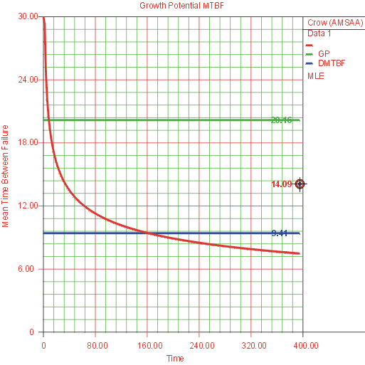
Figure 3: Growth Potential MTBF plot

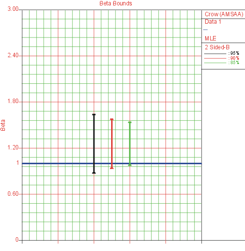
Figure 4: Beta Bounds plot to confirm assumption

RGA also provides pie charts and bar charts for this type of analysis. For example, the bar chart in Figure 5 displays the actual (current) failure rate with the predicted failure rate for all the B modes in the analysis. The chart can also be generated for each individual failure mode. In these charts, the red bar (left) represents the actual failure rate and the green bar (right) represents the failure rate after the fixes have been implemented. From the chart in Figure 5, you can see how each failure mode is contributing to the failure rate of the system. In addition, you can also see how the failure rate for each failure mode is decreasing after the implementation of the fix.

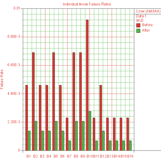
Figure 5: Before and after failure rates for B modes

Figure 6 displays a pie chart of failure modes with categories to represent the steps taken to address the modes: "Type A" will not be addressed. "Type B-Unseen" have not yet appeared in testing but are estimated from the analysis. "Type B-Remain" are failure modes that remain in the system since the corrective actions were not 100% effective and "Type B-Removed" are failure modes that have been removed through corrective actions and their effectiveness. For example, according to this pie chart, almost 29% of the failure modes have not even been observed yet through testing.

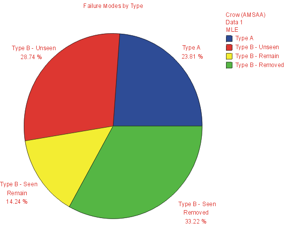
Figure 6: Failure modes pie chart

Repairable Systems Analysis

RGA will also facilitate the analysis of repairable systems data using the Crow (AMSAA) model. For example, you may have a fleet of systems (e.g., a population of cars, motorcycles or ships) such that each of these systems can undergo an overhaul or a repair and be placed back into the field. Analysis of a repairable system using RGA allows you to get an overview of the system without having the large data requirements that would normally be required for system reliability analysis, as in the BlockSim software. You may want to use RGA to track the progress of the system during development and then use BlockSim in accordance with the already known results to gain more detailed information.

In RGA's repairable systems interface, you can enter a start and end time for each system, along with any failure data that you may have for the system. You also have the ability to remove individual systems from consideration in a particular analysis if, for example, the data is not representative of the rest of the population. You can then analyze the data to combine each of these individual systems into a single "superposition" system. The parameters Beta and Lambda for that system, along with the results of the Laplace Trend Test and the Cramer Von Mises goodness-of-fit test, are also displayed for each system individually and for the combined "superposition" system.

Figure 7 displays one of the plots available for repairable systems analysis in RGA. This is the System Operation plot, which displays a timeline of the failures for each of the individual systems, along with the failures for the combined superposition system. You can also generate plots of reliability and unreliability vs. time for the extrapolated superposition system, as shown in Figure 8. Other plots, such as the Cumulative Number of Failures vs. Time plot with either linear or logarithmic axes, are also available.

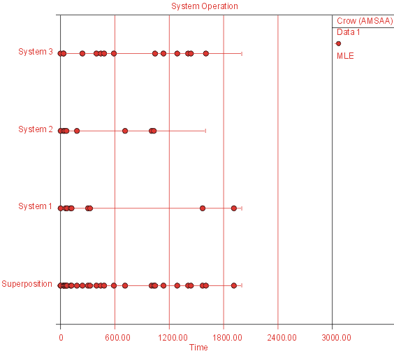
Figure 7: Failures for individual, superposition systems

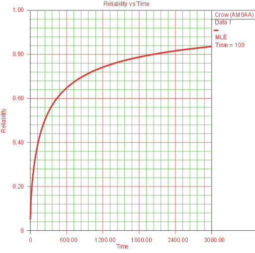
Figure 8: Reliability vs. Time for superposition system

Main Menu

Main Menu

Main Menu

Main Menu

Reliability Growth Analysis and Plots

We have moved ${referer} to www.hbkworld.com

We have moved ${referer} to www.hbkworld.com

We have moved ${referer} to www.hbkworld.com

We have moved ${referer} to www.hbkworld.com

We have moved ${referer} to www.hbkworld.com