The Risks of Using Failure Rate to Calculate Reliability Metrics

A mistake that is often made when calculating reliability metrics is trying to use the failure rate function instead of the probability of failure function (CDF). These two functions, along with the probability density function (pdf) and the reliability function, make up the four functions that are commonly used to describe reliability data. In this article, we will provide a brief overview of each of these four functions, followed by a discussion of how to obtain the pdf, CDF and reliability functions from the failure rate function using ReliaSoft Weibull++. Finally, we will present an example of the error that can be introduced in unreliability calculations by using an approximation based on the failure rate.

Common functions for modeling reliability data

 

The probability density function (pdf) is denoted by f(t). It is a continuous representation of a histogram that shows how the number of component failures is distributed in time. For example, consider a data set of 100 failure times. Histograms of the data were created with various bin sizes, as shown in Figure 1. The pdf is the curve that results as the bin size approaches zero, as shown in Figure 1(c). Note that the pdf is always normalized so that its area is equal to 1. In other words, the histogram shows the number of failures per bin, while the pdf is scaled to show the probability of failure per unit time.

The cumulative distribution function (CDF), also called the unreliability function or the probability of failure, is denoted by Q(t). It represents the probability that a brand-new component will fail at or before a specified time. For example, an unreliability of 2.5% at 50 hours means that if 1000 new components are put into the field, then 25 of those components are expected to fail by 50 hours of operation. The CDF can be computed by finding the area under the pdf to the left of a specified time, or:

Conversely, if the unreliability function is known, the pdf can be obtained as:

The reliability function, also called the survivor function or the probability of success, is denoted by R(t). It represents the probability that a brand-new component will survive longer than a specified time. For example, a reliability of 97.5% at 50 hours means that if 1000 new components are put into the field, then 975 of those components are expected to last at least 50 hours of operation. It can be computed by finding the area under the pdf to the right of a specified time, or:

Conversely, if the reliability function is known, the pdf can be obtained as:

In addition, the reliability function and the unreliability function satisfy the following equation:

The relationship between the pdf, the CDF and the reliability functions are shown in Figure 2.

The failure rate function, also called the instantaneous failure rate or the hazard rate, is denoted by λ(t). It represents the probability of failure per unit time, t, given that the component has already survived to time t. Mathematically, the failure rate function is a conditional form of the pdf, as seen in the following equation:

While the unreliability and reliability functions yield probabilities at a given time from which reliability metrics can be calculated, the value of the failure rate at a given time is not generally used for the calculation of reliability metrics. However, the failure rate versus time plot is an important tool to aid in understanding how a product fails. If the failure rate decreases with time, then the product exhibits infant mortality or early life failures. These types of failures are typically caused by mechanisms like design errors, poor quality control or material defects. If the failure rate is constant with time, then the product exhibits a random or memoryless failure rate behavior. Some possible causes of such failures are higher than anticipated stresses, misapplication or operator error. If the failure rate is increasing with time, then the product wears out. These failures are caused by mechanisms that degrade the strength of the component over time such as mechanical wear or fatigue. An example of an increasing failure rate function is shown in Figure 3.

Using the failure rate to obtain the pdf, CDF and reliability functions

 

If any one of the four functions presented above is known, the remaining three can be obtained. We will focus on how to obtain the pdf, the CDF and the reliability functions from the failure rate function. This will allow us to obtain an expression for the CDF in terms of failure rate that we can use to illustrate the difference between the two functions.

 

The relationship between the pdf and the reliability function allows us to write the failure rate function as:

Therefore, we can establish the relationship between the reliability and failure rate functions through integration as follows:

Then the pdf is given in terms of the failure rate function by:

And the CDF is given by:

A common source of confusion for people new to the field of reliability is the difference between the probability of failure (unreliability) and the failure rate. It can be seen from the preceding equation that the two functions are distinctly different.

Example of error introduced by using failure rate to approximate unreliability

 

To illustrate why it can be dangerous to use the failure rate function to estimate the unreliability of a component, consider the simplest failure rate function, the constant failure rate. Then the unreliability function becomes:

Before computers were widely available, this would have been approximated using a Maclaurin series expansion as:

Taking only the first term (assuming λt is small):

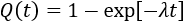
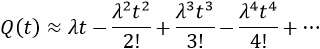
This approximation still exists in some reliability textbooks and standards. Although it was a useful approximation when it was first presented, it applies only for a constant failure rate model and only when the product λt is small.

 

A comparison between the approximation and the actual probability of failure is shown in Table 1, where the value of the failure rate is 0.001 failing/hour (which equates to a mean time to failure of 1000 hours). Assume that the objective of an analysis is to determine the unreliability at the end of a 300-hour product warranty. Using the approximation based on failure rate and time, we would calculate an estimate that is 15% higher than using the unreliability equation itself.

Time	Q(t)	λt	% difference
0	0	0	N/A
50	0.0488	0.05	2.52
100	0.0952	0.10	5.08
150	0.1393	0.15	7.69
200	0.1813	0.20	10.33
250	0.2212	0.25	13.02
300	0.2592	0.30	15.75
350	0.2953	0.35	18.52
400	0.3297	0.40	21.33

 

Table 1: Error introduced by use of approximate unreliability function for constant failure rate case.

Therefore, it is recommended that the CDF should be used for calculations of unreliability at a given time and the time at which a given unreliability occurs, and the failure rate function should be used only as an aid to understand if the model used to fit the data is consistent with the types of failure modes observed or expected for the component.

Conclusion

 

In this article, we discussed the probability density function, unreliability function, reliability function, failure rate function and the relationships between them. A closer look at the failure rate function was presented to illustrate why the unreliability function is preferred over a common approximation using the failure rate function for calculation of reliability metrics. For demonstration purposes, we used Weibull++.