Analysis of Automotive Warranty Data in the Mileage Domain

Please note that the following article — while it has been updated from our newsletter archives — may not reflect the latest software interface and plot graphics, but the original methodology and analysis steps remain applicable.]

Guest Submission - Dustin S. Aldridge, Delphi Corporation

Introduction

Warranty return analysis for automotive components usually centers on looking for trends, manufacturing spills, components built incorrectly but undetected by manufacturing controls, etc., with an eye to managing business costs, maintaining business and assuring success in the marketplace. All are worthwhile aspects of standard business intelligence. Manufacturers desire to address business risks as early as possible. In the automotive industry, an early response to an emerging issue can save a tremendous amount of money, help preserve a business reputation and increase the organizational learning rate. Warranty data is commonly tracked and analyzed in the automotive industry but there are significant business benefits to be gained through swifter reaction to warranty issues. This article highlights an analysis method to better detect potential product issues early in the production cycle, and as the exposure matures this type of analysis can be used to estimate the warranty reserve or measure performance against an established warranty reserve. (A warranty claim does not always represent a product issue or non-conformance to product requirements; hence incidents must be investigated and qualified, with any prediction evaluated in light of data and assumptions to identify the appropriate technical and business actions.) The method involves estimation of the failure distribution from available warranty data coupled with customer usage and application-specific data to more quickly detect and react to potential business risks. To best predict business risk involves a conditional probability analysis to account for the usage truncated warranty risk along with calendar time. Failure distribution analysis is recommended for addition to the standard warranty analysis tool set.

This article promotes an overall philosophy of generating intelligence from automotive warranty data and provides an approach supported by examples of situations where analyzing warranty data led to additional insight in predicting organizational risk and driving earlier action. The method has proven successful in detecting an early transition to a field durability issue, the prediction of warranty risk from a diluted “quality spill” (i.e., a manufacturing problem not detected by existing manufacturing controls), and other issues. [Ref. 1] This process has been employed for some time and has been further enhanced by considering the dual nature of automotive warranty risk related to time and usage, involving a conditional probability analysis. Consistent is the utilization of appropriate life distribution models with clean failure mode data (i.e., classified into unmixed distinct failure modes) as well as a means to rationally consider suspended samples, requiring a suspension strategy. [Refs. 2, 3] In each case, there is an assessment of what data is available and what assumptions need to be made, along with consideration of available statistical and data analysis tools to guide management decisions. The total cost can be predicted from the conditional probability analysis and cost per claim.

Overall Philosophy

The term “intelligence” well describes what is required to create an Early Warning System (EWS) from warranty data. A number of valuable assessment tools have been developed over the years for understanding and detecting spills; however these are primarily reactive. The intent of warranty intelligence tools and systems is to provide the opportunity to discover early indications of unexpected quality and durability problems through the analysis of classified failure mode data. Intelligence also considers No Trouble Found (NTF), Trouble Not Identified (TNI), and other similar acronyms that involve problems resulting from the end product manufacturer integration into a complete system.

Warranty Prediction Based on Failure Distribution Analysis

Warranty returns provide a basis to determine the field use failure distribution. They provide feedback on quality performance and enable predictions regarding quality spill severity. The difficulty in predictions relates to how one accounts for all parts in service. When working in the time domain, this is relatively simple as one has knowledge of the time a part failed and the rest are simply not failed as of the analysis date. The weakness of this is that many failures are not simply a function of time but are more usage-related. Another issue is that often the number of parts actually in service is not known or there is a definite lag time to be accounted for. Failure definitions can be unclear and repair orders can be so non-descriptive that it is difficult to properly classify a failure. These issues must be kept in the mind, but not paralyze an analyst from making reasonable assumptions to enable an analysis with thinking, and discern the intelligence that can be obtained.

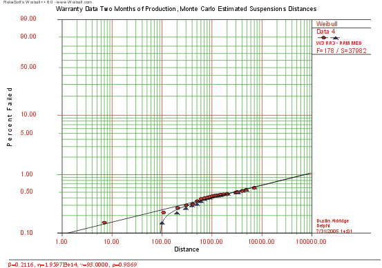
Commonly, failure distribution analysis is not performed, first due to ignorance; second due to a lack of tools; and third, for usage-based analysis, due to the lack of a well-defined method to account for suspended samples. Various methods have been developed for suspensions, such as the Dauser Shift and other reasonable suspension estimation strategies. [Ref. 3]

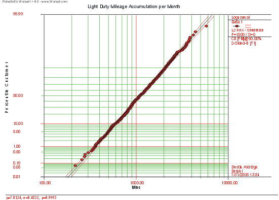
In the automotive industry, time in service is the general parameter of interest. Mileage is known, but commonly not used. If one knows the number of vehicles sold and when, suspensions in time are straightforward for a snapshot. Trends and spikes in time associated with process, design, material or batch issues can be detected and responded to. However, some issues can be missed by not considering usage, which may be design durability-related or the result of a weak sub-population. Mileage accumulation per year across the customer base for light duty vehicles has been studied and documented for many years, where a lognormal distribution similar to Figure 1 (page 19) often models the probability of mileage accumulation levels to customer severity. This distribution is utilized to estimate the mileage for all surviving components in service. The difficulty for accuracy is what the true effective sample size in service is. This can have a large effect on the analysis accuracy early in a product’s life, as a smaller effective sample size will impact the characteristic life, for example, when using a Weibull model. Additionally, using this data one can also consider the portion of the sample that is truncated due to usage, as many customers more quickly fall out on usage than time.

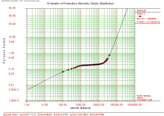
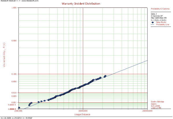
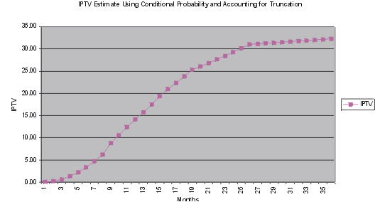
With reasonable data and assumptions to estimate suspension parameters for the sample, a failure distribution model can be calculated with life data analysis software. With further analysis of usage truncation and a conditional probability analysis, one can build a month-to-month risk prediction using the appropriate failure distribution. What options are available will be dependent upon the maturity of the analyzed data. The more mature the data, the higher confidence that can be placed in the analysis. This modeling may lead to additional insight and qualification of the seriousness of the issue or discovery of surprises in the data that traditional methods hide.

Example 1 - Early Warning Detection for Unexpected Durability Risks

To illustrate this methodology, consider a product that was in production for 2 months, with about 38,000 units built and assumed sold. A running prediction of the failure distribution was desired. Using early warranty data, an engineering prediction could be made using a reasonable suspension strategy.

Production was ongoing and thus the sample size was increasingly composed of in-service components. Qualified and mode-specific failure data, production data and mileage accumulation data for the geographic region where the product was being sold were available. To define the suspended sample usage distances, it was assumed that all components produced through the last complete month of production were put into service in the production month, with a mileage accumulation distribution per the application region. Applying a distribution similar to Figure 1 to each month’s production and multiplying by the number of months since production provided an estimate of the accumulated usage for each manufactured part. To make data entry manageable, the resolution of the distance accumulation was set at 200 for all suspended samples (e.g. any distances in the 0 to 200 band were assigned the value of 200). The known warranty failure distances were entered as received with groups of suspended samples occurring at discrete distances to produce the failure distribution seen in Figure 2.

Early in the production cycle when the data was analyzed for a single failure mode with a Weibull model, there is no surprise as we are still clearly in the quality section (characterized by a decreasing failure rate) of the life curve from the analysis in Figure 2. The Weibull slope is much less than 1 and the reliability projection is not alarming at the target life distance. By performing this analysis over time with more components put into service and additional warranty data available, the transition to the constant failure rate zone could be observed. However, after 10 months of maturity, a surprise was discovered. The component moved into an unexpected durability failure zone when analyzed from the mileage perspective with a mixed Weibull analysis modeling the 3 failure regions, as can be seen in Figure 3. What was noteworthy later was that this would not be detected until about 22 months of exposure using traditional analysis methods. Moreover, this prediction proved accurate. Thus an early warning was effectively given 1 year prior to the traditional detection time. An estimate of the warranty expense could be calculated from this analysis as well.

Only by using a customer usage-based suspension strategy and a mixed Weibull model could this transition to a durability failure be seen. Other methods of handling suspensions and simpler failure distribution models hid this behavior. Mixed Weibull allows one to see the quality (decreasing failure rate), the reliability (constant failure rate), as well as the durability sections (increasing failure rate).

Example 2 - Dual Dimensioned Warranty Risk Analysis

Another example involves the aspect of considering the usage and time data truncation for a product. Warranty analysts create graphs (sometimes called "Fan Charts") that show the increase in incidents per thousand vehicles (IPTV) with time. These usually have a characteristic shape due to the reduction in sample size with usage truncation. One can create a fan chart using a past field warranty failure distribution, or one defined from early warranty data, and then calculate the conditional probability of failure for each successive month subtracting out the failed samples. The conditional probability says that given that a certain sample has completed a known exposure, there is a probability that failure will occur in the next usage increment, assuming the defined failure distribution.

Let us assume a product with a 36 month/36,000 mile warranty, a mileage accumulation per month distribution similar to Figure 1, and a warranty incident distribution as shown in Figure 4. Within the Weibull++ software, one can calculate the conditional probability of failure using an embedded spreadsheet function such as shown in Table 1.

Table 1: Conditional Probability of Failure Spreadsheet Function

Performing a usage-based failure distribution analysis after 6 to 12 months enables the joint consideration of usage and time truncation. From this failure distribution, one can calculate for each broad usage group the month-to-month probability of failure and discount those failures that are outside of the usage warranty. An example of this is shown in Table 2.

Table 2: Warranty Failure Distribution Analysis, Mileage Ranges 1 - 2 Months

As time goes on, there will be a portion of vehicles that will be truncated due to exceeding the usage covered by warranty. This results in a loss of sample size and lowers the rate of returns and IPTV. Notice in Table 3 in mileage range 10, we now have about 4 customers out of 1,000 beyond the warranty cut-off point of 36,000 miles.

Table 3: Warranty Failure Distribution Analysis, Mileage Ranges 10 - 11 Months

For customers still in the usage window, we calculate the conditional probability of failure to the next usage range in 1 month. The number of vehicles beyond the truncation point will increase each month where any failures that occur after this point will not be counted by the warranty return system. By month 11, about 15 vehicles have passed the truncation point. This continues until the end of the warranty period, where for this mileage accumulation assumption only about 10% of customers will have less than 36,000 miles by the time-based truncation. Given the resolution of this mileage accumulation distribution, these sample truncations can be seen on the response chart shown in Figure 5 as changes in slope. If one uses early warranty return data, this analysis method may be more representative than an assumed general model as it is based on, and can be updated with, actual product warranty return data.

Conclusion

In the automotive industry, there are benefits in performing life data analysis in the time and usage domains for determining warranty set-aside and predicting business risk. Employing a usage-based scheme is potentially more sensitive and can detect durability issues earlier than a simple time domain analysis, but does require additional information on usage for accuracy. With a good usage model, a joint analysis of time and usage is possible to better predict warranty costs and improves the intelligence from the warranty return system. Plotting the data and thinking upon the results can provide early detection of failure type transitions. This enables improved recognition of potential field issues and estimation of the costs involved. Failure distribution analysis should become part of the standard tool set in warranty analysis. This methodology has proven effective for detection of emerging issues and provides a conservative yet reasonable estimate of business risk.

References

[1] Aldridge, Dustin S., “Prediction of Potential Warranty Exposure and Life Distribution Based Upon Early Warranty Data,” 2006 RAMS PROCEEDINGS. IEEE, Piscataway, NJ, pp 159-164.
[2] ReliaSoft, Life Data Analysis Reference. ReliaSoft Publishing, Tucson, AZ, USA, 1997, pp 55-68.
[3] Abernethy, Robert B., The New Weibull Handbook, Fourth Edition, Robert B. Abernethy, North Palm Beach, FL, USA, 2000, pp 1-3,1-4, 5-9 to 5-11.

About the Author

Dustin Aldridge is a Validation and Test Staff Engineer for the Energy & Chassis Division of Delphi Corporation, located in Juarez, Mexico. He manages product development and validation test programs, lab operations, test equipment engineering, and warranty analysis, supporting multiple product lines. His technical work has concentrated on defining qualification test programs based upon customer usage data and environmental measurements, as well as risk assessment involving multiple integrated aspects of data analysis. He is a member of the SAE Reliability Standards Committee and the Division Director for the Product Reliability Division of IEST. He has published many papers in the environmental test and reliability fields, and represents the U.S. automotive industry for the U.S. delegation to IEC TAG TC56 on Dependability. He can be reached via e-mail at [email protected].