
[Please note that the following article — while it has been updated from our newsletter archives — may not reflect the latest software interface and plot graphics, but the original methodology and analysis steps remain applicable.]
Fatigue failures are failures caused in components under the action of fluctuating loads. They are estimated to be responsible for 90% of all metallic failures since loads on the components usually are not constant but instead vary with time. Fatigue failures occur when components are subjected to a large number of cycles of the applied stress. With fatigue, components fail under stress values much below the ultimate strength of the material and often even below the yield strength. What makes fatigue failures even more dangerous is the fact that they occur suddenly, without warning. The failure begins with a minute crack that is so small that it may not be detected by non-destructive methods such as X-ray inspection. The crack may get initiated by internal cracks in the component or irregularities in manufacturing. Once a crack has formed, it propagates rapidly under the effect of stress concentration until the stressed area decreases so much that it leads to a sudden failure.
Fatigue is a complex phenomenon that is affected by a number of factors, such as the surface finish of the component, environmental effects, heat treatments, presence of stress concentration factors, etc. It is therefore important to carefully analyze components subjected to fluctuating loads so that the desired reliability can be built into these components and over-designed or under-designed components can be avoided.
One of the most common tests for components susceptible to fatigue failures involves running specimens to failure at a constant stress amplitude. Each specimen is loaded in four-point bending and the stress on the specimen is cycled by rotating the specimen. The number of cycles to failure is noted for the stress value. The test is then repeated for different values of stress. It has been found that the cycles to failure, N, versus the stress value, S, follow a straight line when plotted on log-log paper (see Figure 1). The resulting curve is called the Wohler curve or simply the S-N curve. Mathematically, the relationship between the stress and the corresponding cycles to failure (mean value) can be represented as follows:
|
(1) |
where m is the slope of the curve on log-log paper and A is a constant. Once an S-N curve has been obtained from fatigue test data, a design curve is then calculated through the application of various reduction factors and safety factors to reduce allowable stress values at any given point. The design curve is then used to predict product life (in terms of cycles to failure) based on the stress level that the components are expected to encounter in the field.
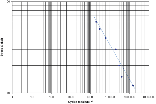
Figure 1: S-N Curve

In this article, we dive into the essential principles and proven techniques that drive product reliability from concept to completion. Many organisations struggle to balance innovation with long-term reliability, often overlooking critical steps that can prevent costly failures down the line.
Although S-N curves are widely used in relation to fatigue failures, they have a number of shortcomings. The first drawback is that the curves are obtained by testing standard specimens under laboratory conditions. Thus the tests are unable to capture the variation of actual components due to factors such as manufacturing defects. The tests also ignore the actual use conditions of the components, which are usually different from the test conditions. Another major drawback is that S-N curves ignore the probabilistic nature of fatigue failures. As demonstrated in Figure 2, the cycles to failure corresponding to a certain stress value may vary considerably even when carefully machined specimens out of the same lot of material are used. The reduction factors used to account for this are an inaccurate way of dealing with this variation. A better approach is to use S-N-P curves, which fully take into account the variation of cycles to failure at each stress level by associating a probability value, P, for the critical cycles at each stress level. The rest of this article describes how to create an S-N-P curve using the ALTA software and the subsequent analyses that are possible with Weibull++ and RENO.
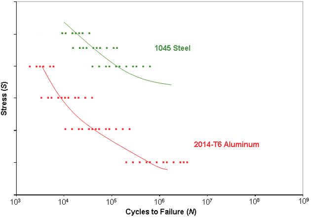
Figure 2: Probabilistic nature of fatigue failures
Consider the case of the fatigue failure of the crankshaft shown in Figure 3, which has failed in pure bending. Assume that the manufacturer wants to be able to accurately predict the reliability of the crankshafts after one year of service at a stress of 20 ksi.
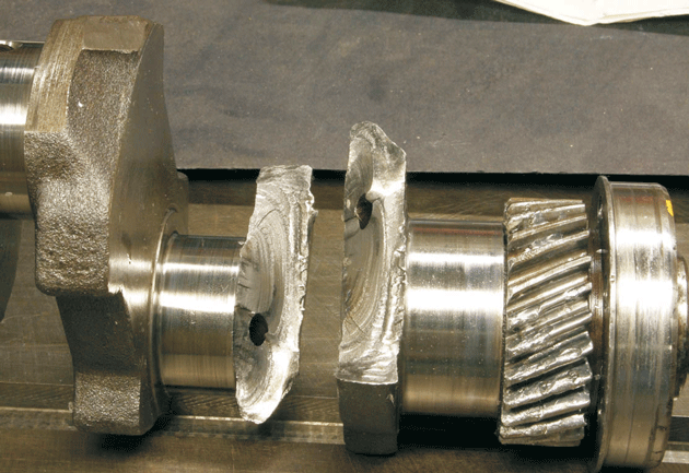
Figure 3: Fatigue Failure of crankshafts
To obtain accurate results, it is decided to randomly select crankshafts from different batches and conduct tests on these units. It is also decided to use accelerated testing to reduce testing time. From Eqn. (1), it can be noted that the relationship between stress, S, and cycles to failure, N, follows the inverse power law. The equation can be re-written and compared to the inverse power law model available in ReliaSoft's ALTA software as follows:
S-N Curve
|
(2) |
Inverse Power Law
|
(3) |
From the comparison of Eqns. (2) and (3), we have K = 1/A and n = m.
It is also known from the theory of fatigue failures that, at each stress, the cycles to failure are lognormally distributed. Thus an ALTA model with the inverse power law life-stress relationship and a lognormal distribution can be used to represent the S-N-P curve. 30 crankshafts are randomly selected and assigned equally to three accelerated stress levels of 39.1 ksi, 63.1 ksi and 79.4 ksi. Table 1 shows the cycles to failure obtained from these tests.
The data of Table 1 are entered into the ALTA software to obtain the S-N-P curve for the fatigue failure of the crankshafts (see Figure 4). The inverse power law - lognormal model with the parameters of σ = 0.575307, K = 1.379346E-13 and n = 4.263146 is found to fit the test data.
Table 1: Cycles to failure obtained from accelerated testing at three stress levels
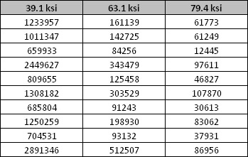
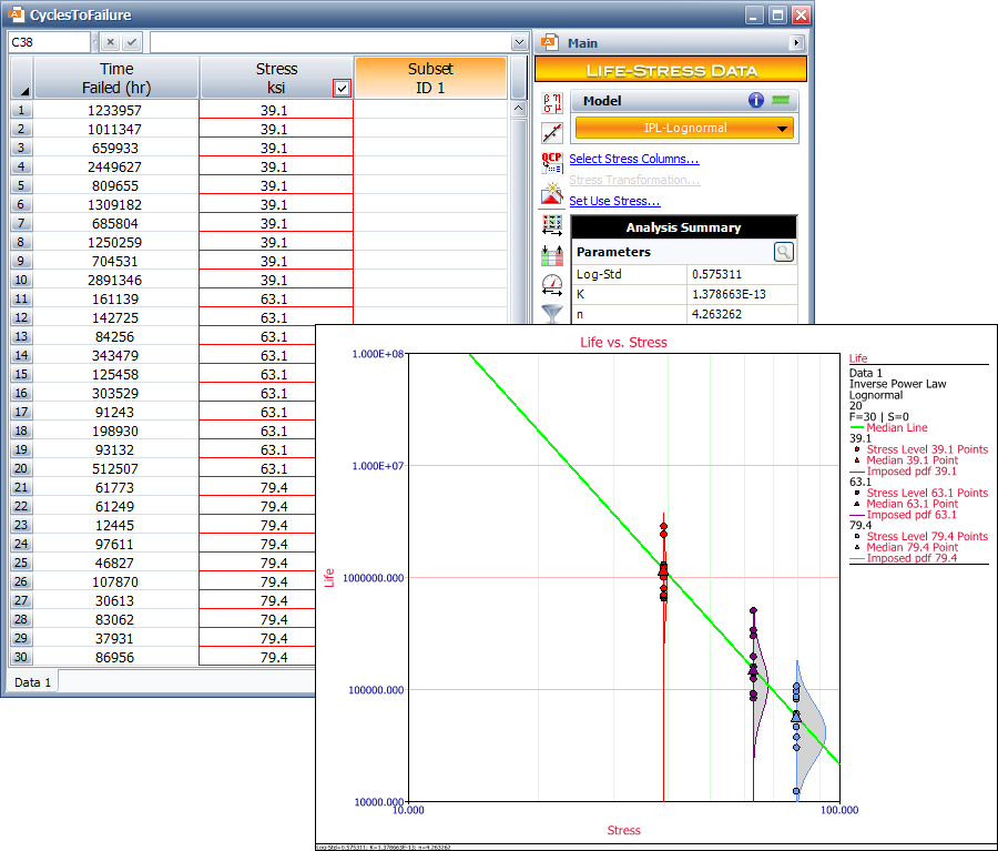
Figure 4: Using ALTA to obtain S-N-P curve from the test data shown in Table 1
The fitted ALTA model can now be used to obtain the distribution of cycles to failure at the stress level of 20 ksi. This is done by setting the "use stress" as 20 ksi in ALTA. Figure 5 shows the distribution of the cycles to failure obtained in this manner.
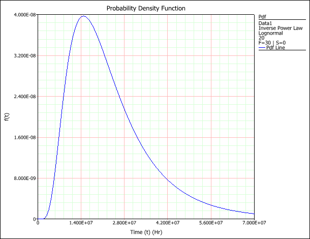
Figure 5: Distribution of cycles to failure at stress = 20 ksi
The manufacturer realizes that different customers will use the crankshaft differently for the one-year period. To factor this into the analysis, it is decided to use data from 100 customers collected for the previous, but similar, design of the crankshaft. It is expected that the use of the crankshaft for the present design under test will be similar to the experience for the previous design. ReliaSoft's Weibull++ software is used to fit a distribution to the cycles used per year for the 100 customers. The resulting usage distribution is the generalized gamma distribution with the parameters of μ = 15.789, σ = 0.4081 and λ = 1.4151 (see Figure 6).
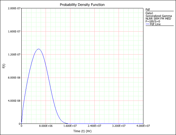
Figure 6: Usage distribution obtained from customer data
The fatigue failure of the crankshafts at the end of one year will not occur as long as the cycles used in one year are less than the value of the critical cycles to failure at a stress of 20 ksi. However, it must be noted that both the cycles used per year and the critical cycles at the stress of 20 ksi are random variables. To obtain the probability that the cycles to failure used will exceed the critical cycles at 20 ksi, the manufacturer needs to compare the distribution of the critical cycles to failure at 20 ksi (lognormal distribution with parameters of m = 16.8409 and σ = 0.5753) and the usage distribution for cycles used per year by the customers (generalized gamma distribution with parameters of μ = 15.789, σ = 0.4081 and λ = 1.4151). This comparison can be done easily in Weibull++ using the stress-strength folio. As shown in Figure 7, the analysis indicates that the reliability of the crankshafts at the end of one year is estimated to be 96.83% (i.e., there is a 3.17% probability that the cycles used by customers in one year would exceed the critical cycles at a stress of 20 ksi).
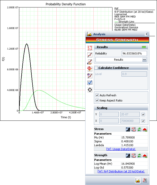
Figure 7: Stress-strength folio to obtain reliability
Although it seems that this analysis is thorough, since it takes into consideration the variation in the crankshafts by testing a random sample and also accounts for the variation in customer usage, it can be further improved. An important point missed in the initial Weibull++ analysis is that the manufacturer assumes that the field stress is constant at 20 ksi. However the stress experienced by the crankshafts will depend upon the loads in the field and the geometrical variation introduced by manufacturing. The next section discusses an analysis approach that accounts for this variation.
The failure of the crankshafts in the present case occurs in bending. The bending stress equation applicable here is:
|
(4) |
where S is the bending stress, M is the bending moment, Z is the section modulus and d is the diameter. It can be seen that the bending stress is a function of two variables: the bending moment, M, and the diameter, d. Both of these variables can be distributed.
The manufacturer is able to obtain the distribution for the bending moment based on the data collected for the previous crankshaft design. Usually such data are collected by attaching appropriate sensors to a few units and recording observations over the component's life. The distribution of the bending moment for the present case is found to be the three-parameter Weibull distribution with parameters of β = 2.6145, η = 616.4701 and γ = 997.7.
The distribution for the diameter is obtained using the tolerance achieved during manufacturing. The tolerance for the diameter section of interest is 1 ± 0.015 inch. Assuming that the diameters are normally distributed, the parameters of the corresponding normal distribution can be determined from the given base dimension and tolerance value. Thus the mean of the assumed normal distribution, which is taken to be the base dimension, is 1 inch. The standard deviation, which is taken to be a sixth of the total tolerance, is 0.005 inch.
Once the distributions of all the variables in the stress equation are known, the distribution of the stress can be obtained using Monte Carlo simulation in Weibull++. Weibull++ generates a number of random values for the bending moment and diameter based on their respective distributions. Then using Eqn. (4), each pair of these random values is used to obtain a value of the bending stress and a distribution is fitted to all such values. (For details see reference [2].) Figure 8 shows the stress distribution obtained in this way.
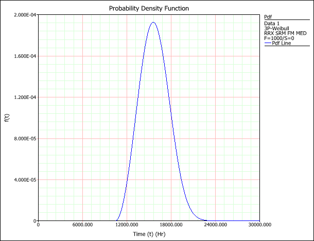
Figure 8: Field stress distribution
To accurately predict the reliability of the crankshafts after one year of service, an advanced model is required that takes into account the S-N-P distribution for the fatigue failure of the crankshafts, the usage distribution for the crankshafts and the distribution of the field stress experienced by the crankshafts. Such a model can be created easily in ReliaSoft's RENO software, as shown next.
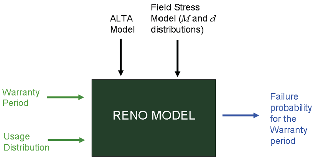
The basis of the RENO flowchart simulation (presented in Figure 9) is the fact that any crankshaft will not fail in a year as long as the cycles used do not exceed the critical cycles at the field stress level.
The RENO model can be used to run a number of simulations to predict the required reliability. During each simulation, the RENO model generates a random bending moment value, M, and diameter value, d, based on the respective distributions to calculate a value of the field stress. Based on this value of the field stress, the ALTA model (S-N-P curve) is used to obtain the corresponding critical cycles to failure. A random value for cycles used is also obtained based on the usage distribution. If the simulated value of the cycles used exceeds the critical cycles to failure then this will result in a failure and is counted as one fatigue failure of the crankshaft. If the simulated value of the cycles used is less than the value of the critical cycles then there will be no failure of the crankshaft. A number of such simulations are run and the count of the total number of failures out of all the simulations is used to arrive at the probability of failure of the crankshafts at the end of one year of service. As shown in Figure 9, this unreliability value is estimated to be 0.0048. Thus the reliability of the crankshafts at the end of one year of service is estimated to be 99.52%. (Note that the increase in the reliability value from the previously obtained value of 96.83% is expected since Figure 8 shows that the majority of field stress values are lower than 20 ksi.)
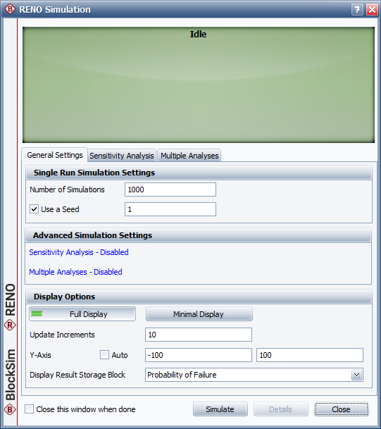
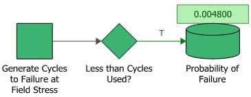
Figure 9: RENO flowchart and simulation settings
The results from the RENO model can be extended to obtain a plot of unreliability at the end of each year of service for a desired time period. This is done by using the option of sensitivity analysis shown in Figure 10. The RENO model applies the usage distribution for one year of service to other periods by simply multiplying the random usage cycles generated by the time period. For example, while calculating the probability of failure of the crankshafts at the end of two years, the generated random value of the cycles used is multiplied by a factor of two.
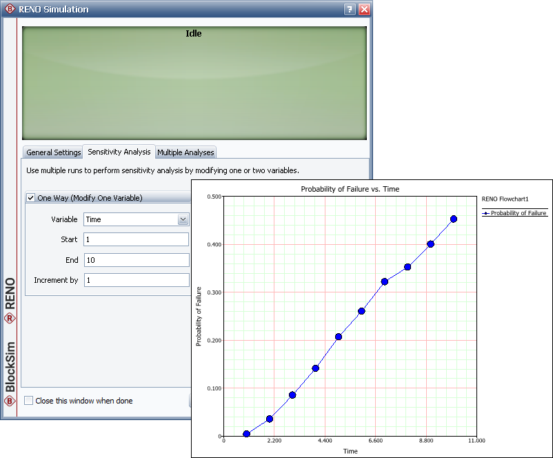
Figure 10: Sensitivity analysis in RENO
In this article we have shown how principles of mechanical design, reliability and customer usage data can be combined effectively to obtain accurate reliability predictions and to design reliability directly into components that are subject to complex failure mechanisms. The combined use of different software tools offered by ReliaSoft makes such analyses easy and efficient.
[1] Kececioglu, D.B., Robust Engineering Design-By-Reliability With Emphasis on Mechanical Components and Structural Reliability, DEStech Publications, Lancaster, PA, 2003.
[2] ReliaSoft, "Engineering Design by Reliability," Reliability Edge, Volume 7, Issue 2, Tucson, AZ, 2006.
[3] ReliaSoft, Accelerated Life Testing Reference, ReliaSoft Publishing, Tucson, AZ, 2007.
[4] Shigley, J.E. and Mischke, C.R., Mechanical Engineering


