Guidelines for Burn-in Justification and Burn-in Time Determination

[Please note that the following article — while it has been updated from our newsletter archives — may not reflect the latest software interface and plot graphics, but the original methodology and analysis steps remain applicable.]

Burn-in is a technique used to increase the quality of components and systems by operating the item under normal or accelerated environmental conditions prior to shipment. If a burn-in procedure is effective, the weak population in the product should be eliminated. Items that are delivered to the consumer are superior to those that would have been delivered without burn-in. The commonly used criteria for evaluating the effectiveness of burn-in testing are: maximum mean residual life, maximum probability of mission success after burn-in, etc. Cost is also often considered as one of the objectives. Costs may include the cost of the burn-in test, cost of warranty claims, cost of items lost to burn-in and cost of failure. Based on different objectives, different burn-in testing strategies should be designed. In the design of a burn-in testing strategy, engineers always ask the following two questions:

Do I need to conduct burn-in testing for my products?
If so, how long does the burn-in testing need to last?

In this article, we will briefly investigate the burn-in techniques and give the answers to these two questions. for more detailed discussion, please see Ref. [1].

Burn-in Justification

First, we should be aware that burn-in testing is not necessary for all the products. In order to benefit from burn-in testing, engineers should collect failure data to decide whether or not burn-in is necessary for the product. In this section, a general procedure for the quantification of a burn-in test is given. It has the following three steps:

Times-to-failure data collection.
Initial data analysis.
Formal parametric data analysis.

Times-to-Failure Data Collection

Times-to-failure data are the key to both burn-in justification and burn-in time determination. Typically, these data can be collected from previous burn-in tests, previous life tests or field failure reports. Depending on how the tests were planned and conducted, or how the field failures were monitored and recorded, the times-to-failure data can be complete failure data or censored data (which includes information about items that did not fail during the observation period, called “suspensions”).

Initial Data Analysis

Before fitting any failure distribution to the collected data, it is better to conduct an initial data analysis. Usually, graphical plotting will give a very straightforward indication about the failure pattern, such as decreasing failure rate (DFR), increasing failure rate (IFR), constant failure rate (CFR) or mixed failure rate (MFR); and whether subpopulations and outliers exist. Weibull probability plots can serve this purpose very well since the Weibull distribution is a flexible distribution. Depending on the value of the shape parameter b, the distribution can describe the failure process with DFR, IFR, CFR and MFR. Two other plots -- mean residual life (MRL) plots and total time on test (TTT) plots -- also can be used to identify the patterns of the failures.

For a Weibull distribution, the probability plot looks like Figure 1.

Figure 1: Weibull Probability Plot

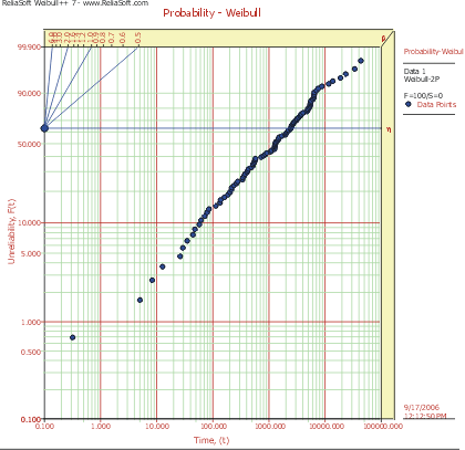
By examining the slope of the plot, the failure rate trend can be obtained. If the slope is greater than 1, the product has an increasing failure rate. If it is less than 1, a decreasing failure rate exists. Further parametric analysis should be conducted after the initial probability plot. By conducting parametric analysis, not only the mean value, but also the confidence interval of the slope can be obtained.

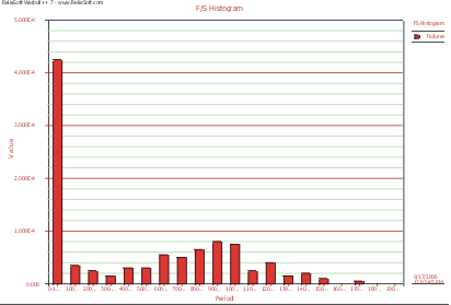
Probability plots and histogram plots can be used to identify whether multiple subpopulations exist in the data. The histogram plot does not require any distribution assumption and is a non-parametric method. For example, a histogram plot may be obtained as shown in Figure 2. This plot provides enough evidence to show that there are two subpopulations in the collected failure data.

Figure 2: Histogram Plot of the Failure Data

In the probability or histogram plot, if any points appear to be outliers, then the test procedure and data records need to be checked. Any confirmed outliers should be removed from the original data set before further analysis. Otherwise, such observations should be kept in the data set.

Formal Parametric Data Analysis

The initial data analysis in the previous section provides an indication about the failure pattern and subpopulation behavior, which facilitates the selection of a proper model for describing the failure process during burn-in. In this section, we will discuss the two commonly used mathematical models for the failure process during burn-in. One is the single population Weibull model and another is the mixed-Weibull model. Since the exponential distribution is a special case of the Weibull model, the mixed-exponential model falls under the mixed-Weibull family. The mixed-Weibull model can describe the reliability bathtub curve very well. Another type of model called the "bathtub curve family" can also be used to describe the bathtub curve and the burn-in failure process. For details, please refer to Ref. [1].

Single Population Weibull Model

This model is also called the 2-parameter Weibull. Its probability density function is given by:

The failure rate function is given by:

where β is the shape parameter and η is the scale parameter. From Eqn.(2) we can see that if β is less than 1, the failure rate will decrease with the time and if β is larger than 1, the failure rate will increase with time. If β is equal to 1, the failure rate is a constant value. The use of β to determine the burn-in time is illustrated later in this article.

Mixed-Weibull Model

In this article, we only consider the 2 population mixed-Weibull model or bimodal mixed-Weibull model. A 2 population mixed-Weibull model can be used to describe a population with two different distributions. A freak population represents the weak or substandard components or assemblies with strength values much smaller than the specified limits. A main population represents a subpopulation of the strong or standard components or assemblies with strengths around the specified limits. The weak population is usually caused by defects in the manufacturing process and the lack of quality control. The probability density function for the mixed-Weibull model is shown in Figure 3.

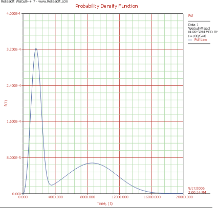
Figure 3: Probability Density Function of a Bimodal Distribution

For the bimodal mixed distribution, it is expected that an effective burn-in will eliminate those substandard components governed by the freak strength distribution. The cumulative distribution function of the bimodal Weibull distribution is given by:

Where:

and

and p is the fraction of the freak population in the total population.

Parameter Estimation and Model Validation

Once a mathematical model has been selected to describe the failure data, the next task is to estimate the model parameters. Basically, the parameter estimation methods for the failure time distribution can be divided into the following two categories: 1) Graphical Methods and 2) Analytical Methods. ReliaSoft's Weibull++ software provides many analytical methods for parameter estimation, such as Maximum Likelihood Estimation (MLE), Least-Squares Estimation (LSE) and Bayesian method.

After the parameters have been estimated, the next step is to validate whether or not the selected model fits the data. Using a combination of goodness-of-fit tests and engineering judgment, different models can be tried until the one that provides the most satisfactory fit is found. A goodness-of-fit test is a very effective tool to check the validity of the model. The Distribution Wizard in Weibull++, which performs three different goodness-of-fit tests and ranks each distribution according to their combined performance on these tests, can be used for selecting the best fit model from a statistical perspective. For more detail, please see Ref. [2]. Notice that engineering judgment is an integral part of the model selection process as well.

Burn-in Objective and Time Determination

After estimation of the model parameters and validation of the obtained model, the next task is to determine the "optimum" burn-in time. "Optimum" is related to an objective function. A burn-in time that is optimum to one objective may not also be optimum to other objectives. Therefore, it is necessary to develop the appropriate objective function first before proceeding to determine the burn-in time length.

The objectives can be:

A specified (or the minimum) failure rate at the end of burn-in.
A specified (or the maximum) post-burn-in mission reliability.
The expected minimum cost.
The elimination of the freak population.
A specified (or the maximum) post-burn-in mean residual life.

Analysts may also define their own objectives. In the following discussion, we will present examples of determining burn-in time based on the failure model and a given objective. More detailed discussion can be found in Ref. [1].

Burn-in Time Corresponding to a Specified Failure Rate Goal

This method is usually used when the product has a decreasing failure rate. The estimated failure rate function is as given in Eqn. (2). Let the failure rate goal be λ_G, then:

From Eqn. (4), one can solve the corresponding burn-in time t_b by:

equation

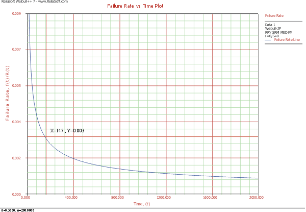
The burn-in time can also be easily identified by looking at the failure rate plot in Weibull++7. For example, for a Weibull distribution with β = 0.5 and η = 200, the failure rate plot is as given in Figure 4. If the post-burn-in failure rate goal is 0.003, then from Figure 4, it can be seen that the corresponding burn-in time is 147.

Figure 4: Failure Rate Plot for Weibull Distribution with Decreasing Failure Rate

Burn-in Time Corresponding to a Mission Reliability Goal

This method can be used for both the single Weibull and the mixed-Weibull distribution. For a mission time t after t_b hours of burn-in, the mission reliability is given by:

For the single Weibull model with decreasing failure rate:

If R_G, β, η and the mission time t are given, then from Eqn. (7), one can solve for the corresponding burn-in time t_b using the non-linear equation root finder in Weibull++.

For the bimodal mixed-Weibull model, Eqn. (6) becomes:

and t_b can be solved for using the non-linear equation root finder or the tabular approach of Table 1 can be used. For example, let p = 0.366, β₁ = 0.57, η₁ = 530, β₂ = 1.82 and η₂ = 5900. Assume that the reliability goal is 0.99 and the mission time is 50 hours. Using the conditional reliability function provided in Weibull++, we get the results shown in Table 1.

Table 1: Mission Reliability for a Given Burn-in Time

Burn-in Time	Reliability Goal	Burn-in Time	Reliability Goal
50	0.96320264	550	0.989308
100	0.97258375	600	0.989803
150	0.97758019	*650*	0.990222
200	0.98079726	700	0.990577
250	0.98307278	750	0.990880
300	0.98477570	800	0.991137
350	0.98609860	850	0.991356
400	0.98715362	900	0.991542
450	0.98801127	950	0.991700
500	0.98871850	1000	0.991832

From Table 1, we can see that the burn-in time of 650 will meet the reliability goal. The exact numerical solution of Eqn. (8) is 646.85 hours. Thus the result obtained from Table 1 is very close to the exact numerical solution.

Burn-in Time Corresponding to the Expected Minimum Cost

This method is usually used for the single Weibull distribution with the shape parameter β < 1. Weibull++ 7 has a template that can be used to find the optimum burn-in time by minimizing the expected cost. More detailed discussion on this can be found in Ref. [3].

Burn-in testing requires testing all units for the designated time; therefore, it increases production lead time as well as costs. The following expected cost model addresses the trade-off between the costs of conducting the burn-in and the cost of failures following burn-in. Let:

C_b = cost per unit time for burn-in testing
C_f = cost per failure during burn-in
C_o = cost per failure when operational
t_b = length of burn-in testing
t = operational life of the units

Assume n units are placed under burn-in testing. Those that fail during burn-in are discarded and the surviving units continue to be operational. The expected number of failures during burn-in is n[1-R(t_b)]. The expected number of operational failures is:

The expected total cost is:

The expected cost per unit for the Weibull distribution is:

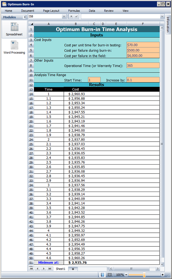
For a Weibull distribution with β = 0.529, η = 168, Cb = $70, Cf = $500 and Co = $4,000, based on Eqn. (11), applying the Burn-in Template provided by Weibull++ 7, we get the plot shown in Figure 5. By examining the cost curve, the optimum burn-in time that results in the minimal expected cost can be located. This time is 2.5 hours.

Figure 5: Burn-in Test Report

Burn-in Time Corresponding to Eliminating the Freak Population

This method is used when there is more than one population in the failures, especially for the data that can be modeled by a bimodal mixed Weibull distribution. Many companies want to eliminate the freak population before they ship the product. Burn-in can efficiently meet this goal since the freak population usually has a relatively short life. Assuming the burn-in time to be t_b, the new cumulative distribution function, F_n(t), describing the remaining part of the distribution is given by:

where F(t) is given in Eqn. (3).

If the burn-in for t_bhas been carried out so that the freak subpopulation has been more or less eliminated, then:

Thus Eqn. (12) becomes:

Eqn. (14) can be used to calculate the probability of failure of the population that survived the burn-in test. the burn-in time can be determined by a simple graphical method.

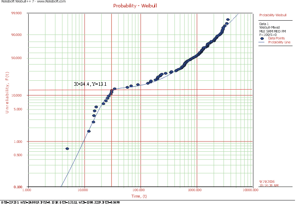
From the parameters of the fitted model, we know that the proportion of the weak population is p = 13.1%. Therefore, we locate the point with the unreliability equal to 0.131 in the probability plot and find the corresponding time is 34.4. This also can be done using the Quick Calculation Pad (QCP) tool in Weibull++. The burn-in time 34.4 will eliminate most units in the weak population.

Figure 6: Bimodal Mixed-Weibull Probability Plot

Burn-in Time Corresponding to a Specified Post-Burn-in Mean Residual Life

The definition of mean residual life (MRL) is: given that an item is of age t, the remaining life after age t, which is a random variable, is called the residual life. The expected value of this random residual life is called the mean residual life at age t. In general, MRL is a function of age t. MRL can be calculated by:

More details about MRL can be found in Ref. [1]. A burn-in procedure is justified for the case when the products have an increasing MRL or when the products exhibit an increasing MRL first and then the MRL starts decreasing. Because these units exhibit a decreasing failure rate during their early life period, burn-in before delivery will eliminate the defective units from the population and increase the residual life of the delivered units.

Though both the failure rate function at age t, λ(t) and the MRL function at age t, are conditional on the survival of an item to age t, m(t) provides information about the whole interval after t, while λ(t) provides information only about a small interval after age t, which is the interval (t, t + Δt).

The empirical MRL function can be calculated by:

The following example illustrates how to use the empirical MRL plot to determine a suitable burn-in time. Consider the failure data from a life test of 4500 hours on N = 150 electronic components shown in Table 2.

Table 2: Failure Data for MRL Calculation

Failure Order	Number in State	State F/S	State End Time	MRL
1	1	F	100	33033
2	1	F	200	34035
3	1	F	250	35262
4	2	F	420	36896
5	3	F	588	40382
6	1	F	708	49180
7	1	F	1044	52394
8	2	F	2892	52952
9	2	F	3396	31121
10	3	F	3997	29660
11	1	F	4165	33283
12	1	F	4500	44220
-	131	S	4500

Applying Eqn. (16) to the data in Table 2, the empirical MRL at any specified age t between t_k and t_k+1 is:

For example, if t = t₁₀ = 3997, then the estimated m(t) is:

The empirical MRL plot is shown in Figure 7.

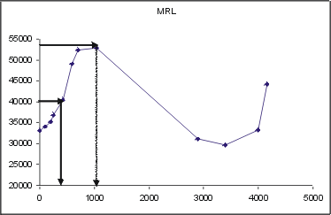
Figure 7: Example of Empirical MRL Plot

If the goal for MRL after burn-in is 40000 hours, then from Figure 7, it can be seen that the corresponding burn-in time is about 400 hours. It can also be observed from the plot that the maximum achievable MRL is about 53000 and the corresponding burn-in time is about 1000 hours.

Conclusion

In this article, the issues of whether to conduct a burn-in test and how to determine an optimum burn-in time were discussed. The article shows that analyzing the field and test failure data is very important. The analysis results can help decide whether a burn-in program will be beneficial. Depending on the objective there are different ways of determining the burn-in length. In this article, five commonly used objectives and the corresponding burn-in time determination methods were discussed.

Note that if a burn-in test is to be conducted at a stress level that is different from that at which the times-to-failure data were collected, then an acceleration factor needs to be determined for converting a burn-in time at one stress level to that at another stress level. The acceleration factor can be calculated using the ALTA 7 software that will soon be released by ReliaSoft.

References

[1] Kececioglu, D. and Sun, F. B., Burn-In Testing, Its Quantification and Optimization, Prentice Hall, New Jersey, 1997.
[2] ReliaSoft, Life Data Analysis Reference, 2005.
[3] Ebeling, C., An Introduction to Reliability and Maintainability Engineering, McGraw-Hill, 1997.

[Editor's Note: In the printed edition of Volume 7, Issue 2, the data for the second column of Table 1 was printed incorrectly. This has been corrected in this online version. We apologize for any inconvenience.]

Main Menu

Main Menu

Main Menu

Main Menu

Guidelines for Burn-in Justification and Burn-in Time Determination

Burn-in Justification

Times-to-Failure Data Collection

Initial Data Analysis

Figure 1: Weibull Probability Plot

Figure 2: Histogram Plot of the Failure Data

Formal Parametric Data Analysis

Single Population Weibull Model

Mixed-Weibull Model

Figure 3: Probability Density Function of a Bimodal Distribution

Parameter Estimation and Model Validation

Burn-in Objective and Time Determination

Burn-in Time Corresponding to a Specified Failure Rate Goal

Figure 4: Failure Rate Plot for Weibull Distribution with Decreasing Failure Rate

Burn-in Time Corresponding to a Mission Reliability Goal

Table 1: Mission Reliability for a Given Burn-in Time

Burn-in Time Corresponding to the Expected Minimum Cost

Figure 5: Burn-in Test Report

Burn-in Time Corresponding to Eliminating the Freak Population

Figure 6: Bimodal Mixed-Weibull Probability Plot

Burn-in Time Corresponding to a Specified Post-Burn-in Mean Residual Life

Table 2: Failure Data for MRL Calculation

Figure 7: Example of Empirical MRL Plot

Conclusion

References

We have moved ${referer} to www.hbkworld.com

We have moved ${referer} to www.hbkworld.com

We have moved ${referer} to www.hbkworld.com

We have moved ${referer} to www.hbkworld.com

We have moved ${referer} to www.hbkworld.com