[Please note that the following article — while it has been updated from our newsletter archives — may not reflect the latest software interface and plot graphics, but the original methodology and analysis steps remain applicable.]
Successful manufacturers recognize that it is crucial to have sufficient and accurate time-to-failure data in order to make accurate estimates about the expected longevity of their products. However, for many manufacturers in today's marketplace, it is difficult or impossible to obtain failure data for their products in a cost-effective manner prior to product release. They may be unable to test new product designs to failure under normal operating conditions because their products have long lifetimes, because the time between design and product release is too short, or for a variety of other reasons.
The analysis of degradation data is one way to overcome these obstacles to obtain the information required to make effective business decisions regarding warranty periods and/or to demonstrate that the product meets the reliability specifications of the customer. Degradation analysis involves the measurement of the degradation of a product, where the degradation can be directly related to the expected failure of the product. This information is then used to estimate the eventual failure time for the product.
Degradation analyses can be performed on data obtained under normal use conditions or under accelerated stress conditions. ReliaSoft Weibull++ software allows you to extrapolate time-to-failure information from degradation data obtained under use conditions and ALTA allows you to take accelerated stress levels into account. This article presents the methodology behind degradation analysis and examples of its application under both normal and accelerated conditions.
In order to use degradation data to estimate times-to-failure for the product, the degradation factor that is being measured must be directly related to a failure mechanism for the product and there must be a definite level of degradation at which a failure is said to have occurred. For example, if the wear of a tire tread is directly related to the eventual failure of the tire and the degree of wear that results in the failure of the tire can be defined, you can use degradation analysis to estimate time-to-failure data for the product.
In some cases, it is possible to directly measure the degradation over time, as with the wear of brake pads or with the propagation of crack size. In other cases, it may not be possible to directly measure the degradation without invasive or destructive measurement techniques that would directly affect the subsequent performance of the product. In such cases, the degradation can be estimated through the measurement of certain performance characteristics, such as using resistance to gauge the degradation of a dielectric material. Performance and degradation data are analyzed in a similar manner.
Once you have determined the degradation factor that eventually results in product failure, devised a method to measure the degradation and defined the level of degradation at which the product is considered to be "failed," the next step is to measure the degradation for multiple units over time and record the results. As with conventional reliability data, the amount of certainty in the results is directly related to the number of units being tested. With this information, it is a relatively simple matter to use basic mathematical models to extrapolate the degradation measurements over time to the point at which the product is expected to fail. You can then analyze these estimated failure times with standard life data analysis techniques and obtain standard reliability results, like mean time, warranty time and B(X) life.
The linear, exponential, power and logarithmic models are basic mathematical models that can be used to extrapolate the degradation measurements to the defined failure level in order to estimate the failure time. These models have the following forms:
| Linear: | |
| Exponential: | |
| Power: | |
| Logarithmic: |
In these formulations, y represents the performance, x represents time and a and b are model parameters to be solved for. Once the model parameters ai and bi are estimated for each sample i, a time (xi) can be extrapolated that corresponds to the defined level of failure y. The computed xi can then be used as times-to-failure points in subsequent life data analysis. As with any sort of extrapolation, you must be careful not to extrapolate too far beyond the actual range of data in order to avoid large modeling errors.
The following examples demonstrate the use of degradation data to extrapolate failure times and determine the B(10) life for a product. The first example involves data obtained under normal use conditions and analyzed in Weibull++ 6. The second example involves data obtained under accelerated stress conditions and analyzed in ALTA 6. The underlying degradation analysis principles are the same in both cases.
Suppose that five turbine blades were tested for crack propagation under normal use conditions. The test units were cyclically stressed and inspected every 100,000 cycles for crack length. Failure is defined as a crack of length 30mm or greater. The test results are presented in Table 1.
You can use degradation analysis with an exponential model for failure extrapolation to determine the B(10) life (the time at which 10% of the products will fail) for the turbine blades. The first step is to solve the equation,
![]()
for a and b for each of the test units. Using regression analysis, Weibull++ calculates these values for each of the test units. These values can then be substituted into the underlying exponential model, solved for x or:
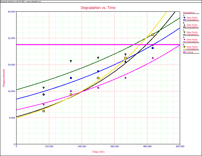
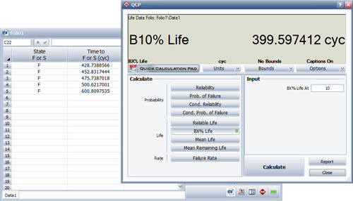
Using the values of a and b with y = 30, you can calculate the point at which the length is expected to reach 30mm for each sample unit. A plot of the degradation analysis is presented in Figure 1 and the extrapolated cycles-to-failure are shown in the Weibull++ Degradation Analysis utility in Figure 2.
|
FIGURE 1: PLOT OF DEGRADATION RESULTS FROM WEIBULL++ |
These cycles-to-failure can now be analyzed in the conventional manner. Assuming a two-parameter Weibull distribution and using the MLE estimation method, the distribution parameters for the extrapolated data are calculated as
![]()
= 8.0552 and
![]()
= 519.5559. Using this analysis, the B(10) life is calculated to be 392,920 cycles, as shown in Figure 2.
|
FIGURE 2: EXTRAPOLATED CYCLES-TO-FAILURE DATA AND QCP RESULTS FROM WEIBULL++ |
Consider a chemical solution that degrades with time. A quantitative measure (QM) of the quality of the product can be obtained and this measure is said to be around 100 when the product is first manufactured and decreases as the product ages. Products with a QM equal to or lower than 50 are considered to be "out of compliance" or failed. The "shelf life" for the product is defined as the time at which 10% of the products will have a QM that is out of compliance.
The product's normal use temperature is 20 degrees Celsius (or 293K) and engineering analysis has indicated that the QM has a higher rate of decrease at higher temperatures. A quantitative accelerated life test was performed to determine the shelf life of the product. Fifteen samples were tested, with five samples in each of three temperature environments: 323K, 373K and 383K. Once a month for seven months, the QM for each sample was measured and recorded. Although none of the samples were out of compliance at the end of seven months, the QM was observed to degrade over time.
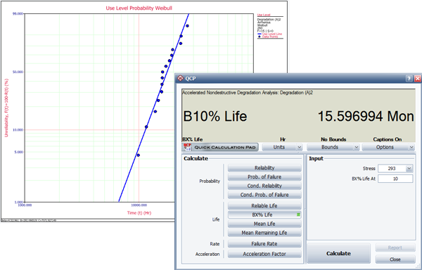
You can use the ALTA 6 Degradation Analysis utility to extrapolate times-to-failure data points at each accelerated stress level, based on the accelerated degradation data and the exponential degradation model. When the extrapolated data points are transferred to an ALTA Data Folio, you can obtain standard reliability results, like the B(10) life, and various probability, life vs. stress and other plots. The use level probability plot and the QCP results for the B(10) life calculation are displayed in Figure 3. Based on this analysis, the projected shelf life for the product (the time at which 10% of the products are expected to fail) is 15.6 months.

This will bring together HBM, Brüel & Kjær, nCode, ReliaSoft, and Discom brands, helping you innovate faster for a cleaner, healthier, and more productive world.
This will bring together HBM, Brüel & Kjær, nCode, ReliaSoft, and Discom brands, helping you innovate faster for a cleaner, healthier, and more productive world.
This will bring together HBM, Brüel & Kjær, nCode, ReliaSoft, and Discom brands, helping you innovate faster for a cleaner, healthier, and more productive world.
This will bring together HBM, Brüel & Kjær, nCode, ReliaSoft, and Discom brands, helping you innovate faster for a cleaner, healthier, and more productive world.
This will bring together HBM, Brüel & Kjær, nCode, ReliaSoft, and Discom brands, helping you innovate faster for a cleaner, healthier, and more productive world.
This will bring together HBM, Brüel & Kjær, nCode, ReliaSoft, MicroStrain and Discom brands, helping you innovate faster for a cleaner, healthier, and more productive world.