One-Way Analysis of Variance (ANOVA) and Reliability DOE: Applying Reliability DOE Techniques to Investigate Effects on Product Life

[Please note that the following article — while it has been updated from our newsletter archives — may not reflect the latest software interface and plot graphics, but the original methodology and analysis steps remain applicable.]

 

In a previous article [1], we provided an introduction to the concept of Design for Reliability (DFR). With the DFR approach, the organization implements an entire set of tools and practices that support product and process design in order to ensure that customer expectations for reliability are fully met throughout the life of the product with low overall life-cycle costs.

 

Within the DFR concept, the methodology of Design of Experiments (DOE) can be applied in the design and manufacturing stages to improve product reliability. It can be used to systematically investigate the variables (factors) that influence the life of the product, thereby providing the analyst with information that can be used to improve reliability. The analysis can also be used in the production stage to estimate product reliability for predictions (e.g. warranty predictions). This can be done as a two-step process in which DOE is used first to identify the factors that affect product reliability. Then the principles of accelerated life testing analysis can be used to create a model that enables predictions.

 

This article illustrates how DOE techniques can be applied to reliability analysis to investigate the effect of a particular characteristic on the life of a product. It initially presents the traditional analysis approach referred to as one-way ANOVA. It then contrasts this analysis to one factor reliability DOE analysis, which is a more suitable approach for dealing with investigations involving life data. If the investigated characteristic is a stress affecting the life of a product, then a prediction model can be built based on the results of the one factor reliability DOE analysis. The final sections of the article illustrate the procedure to build such a reliability model using accelerated life testing analysis (ALTA) principles.

 

One-Way ANOVA

 

Analysis of Variance (or ANOVA) refers to the procedure of partitioning the variability of a data set to conduct various significance tests. In experiments where only a single factor is investigated, the analysis of variance is referred to as one-way ANOVA. The basic assumption in applying ANOVA is that the response is normally distributed. The variance of the response is divided into the variance that can be attributed to the investigated characteristic (or factor) and the variance that can be attributed to the randomness that is seen to occur naturally for the response. The former is referred to as the treatment mean square, MS_TR, while the latter is referred to as the error mean square, MS_E. A ratio of the two terms is used to conduct the F test.

 

(1)

 

The ratio of Eqn. (1) is referred to as the F ratio. It is assumed that if the investigated factor does not affect the response, then MS_TR will not be significantly different from MS_E. In such cases, the F ratio will be close to a value of 1 and will follow the F distribution. On the other hand, if the investigated factor does affect the response, then the F ratio will not follow the F distribution and the p value corresponding to the F ratio will indicate this. (For additional details on one-way ANOVA and the calculation of the p value, refer to [2].)

 

Difficulties in Applying One-Way ANOVA to Life Data

 

The application of one-way ANOVA to a response requires the assumption that the response is normally distributed. However, this assumption seldom applies to life data, which are typically well modeled by the exponential, Weibull or lognormal distributions. Additionally, ANOVA cannot handle suspensions or interval data. To apply ANOVA to censored data, the suspensions are usually treated as failure times and the mid-points of the interval data are taken as the times-to-failure. Most of the time, however, such assumptions are not valid and may result in misleading conclusions.

As an example, consider a component whose life has been found to follow the Weibull distribution. The component is tested at three temperatures to investigate whether the operation temperature has an effect on the life of the component. The test is run for 1000 hours and all components that have not failed by this time are treated as suspensions. Table 1 shows the data set recorded from the test, where "F" indicates a failure and "S" indicates a suspension.

 

 

A one-way ANOVA can be conducted to investigate whether the life of the component is statistically different at the three operation temperatures. As mentioned above, in order to conduct a one-way ANOVA for this data set, it has to be assumed that the life of the component follows the normal distribution. Further, all suspensions in Table 1 have to be treated as failure times or have to be ignored.

Using these two assumptions, the data can be entered into ReliaSoft Weibull++ software as shown in Figure 1 and the software generates the "ANOVA Table" shown in Figure 2. It can be noted from the figure that the value of the coefficient of multiple determination, R² (shown as R-sq in the Weibull++ results), is about 51%. This indicates that the ANOVA model is not a good fit for the present data [2]. Figure 3 displays the residual plot obtained from the analysis. The plot shows that the residuals do not follow the normal distribution well, indicating that the normal distribution assumption is not applicable for the data. Consequently, the results obtained from the one-way ANOVA are not dependable.

 

Figure 1: Data entered for one-way ANOVA in Weibull++

 

Figure 2: Results from the one-way ANOVA

 

Figure 3: Residual probability plot for the one-way ANOVA

 

Reliability DOE Analysis

 

Weibull++ offers an alternative analysis approach, called reliability DOE analysis, which can be used to overcome the problems associated with applying ANOVA to life data. In reliability DOE analysis, instead of using the F ratio, which is based on the normal distribution assumption, the likelihood ratio is used, which does not require such an assumption. The likelihood ratio is calculated using the likelihood function, which also takes into account suspensions and interval data. Therefore, the issues associated with applying one-way ANOVA to life data are well taken care of by using one factor reliability DOE analysis, as illustrated next.

 

It was mentioned previously that the life of the component in this example is well modeled by the Weibull distribution. The probability density function for the Weibull distribution can be written as:

 

(2)

 

where:

 

• t represents the times-to-failure.

• β represents the shape parameter of the Weibull distribution.
• η represents the scale parameter of the Weibull distribution.

 

The scale parameter, η, represents the time by which 63.2% of the population is expected to fail. It is also is referred to as the life characteristic because it represents a characteristic point of the Weibull distribution. The life characteristic will change based on the underlying distribution assumed for the life data.

The model used in the one factor reliability DOE approach is based on the life characteristic. It is known that a factor with L levels will have (L - 1) independent effects if the zero sum constraint is used [2]. Therefore in this example, the factor (operation temperature) with three levels (326K, 336K and 346K) can be used to express the life characteristic using two independent effects as follows:

 

(3)

 

where:

 

• η represents the life characteristic for the Weibull distribution.
• x₁ and x₂ are the variables representing the two independent effects of the factor.
• α₀ is the intercept term.
• α₁ is the coefficient for the first independent effect, x₁.
• α₂ is the coefficient for the second independent effect, x₂.

 

Note that in Eqn. (3), the natural logarithmic transformation has been applied to the life characteristic. The reason for this is that η cannot take negative values as it represents product life, which is non-negative.

 

The variables, x₁ and x₂, representing the two independent effects, take the following values for the three levels of the operation temperature:

 

 

 

 

The log-likelihood function for a data set following the Weibull distribution is written as:

 

(4)

 

where:

 

• i represents the level of the factor.
• F represents the number of failures at the i^th level of the factor.
• S represents the number of suspensions at the i^th level of the factor.

 

The value of the life characteristic at the i^th level can be substituted into Eqn. (4) using Eqn. (3). The value of η_i to be substituted can be obtained as follows:

 

(5)

 

In Eqn. (5) the values of x₁ and x₂ used are based on the previously mentioned coding scheme for the three levels of the factor. The overall log-likelihood function for the data will be:

 

(6)

 

Eqn. (6) is used to obtain the maximum likelihood estimates of the parameters β, α₀, α₁ and α₂. This is done by taking the partial derivatives of the overall likelihood function Ln(LKV) with respect to the model parameters and then setting the resulting equations to zero.

Once the maximum likelihood estimates of the parameters are known, a test to check the significance of the factor can be carried out using the likelihood ratio. If the factor, operation temperature, does not affect life significantly, then the life characteristic, η, will be the same at all levels of the factor. In other words, the levels of the factor will not affect η; consequently the coefficients α₁ and α₂ of Eqn. (2) will be zero. In this case, the equation for η will be:

 

(7)

 

Eqn. (7) is referred to as the reduced model.

If change in the level of the factor affects life then the coefficients α₁ and α₂ will have non-zero values and the equation for ηwill be:

 

(8)

 

Eqn. (8) is referred to as the full model.

The likelihood ratio used in one factor reliability DOE analysis is based on the ratio of the log-likelihood value corresponding to the reduced model, Ln(LKV0), and the log-likelihood value corresponding to the full model, Ln(LKV). The likelihood ratio is defined as follows:

 

(9)

 

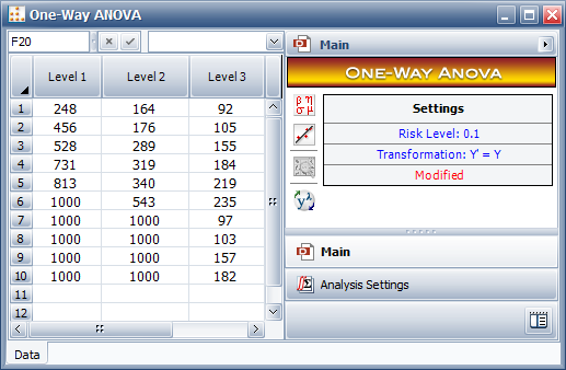
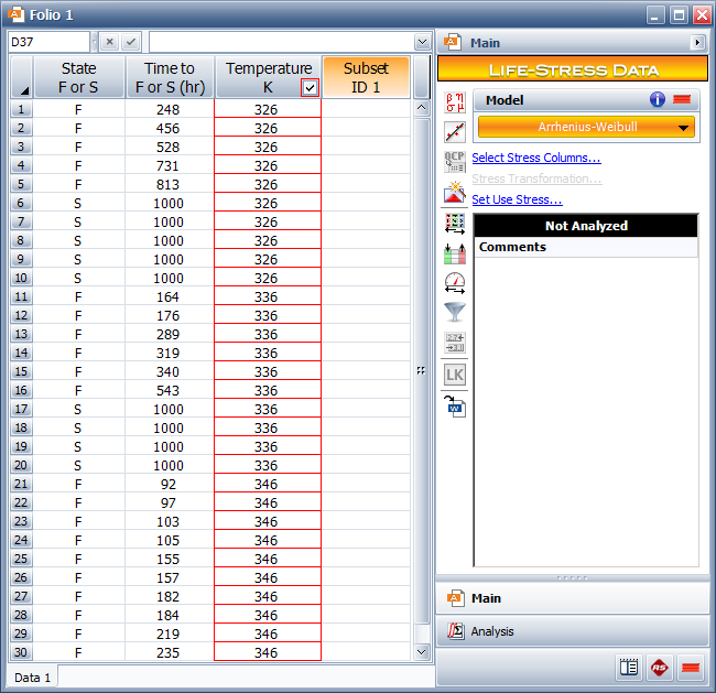
Eqn. (9) is analogous to Eqn. (1) used in one-way ANOVA. If the parameters α₁ and α₂ are zero, then the likelihood ratio, LR, follows the chi-squared distribution with (L - 1) degrees of freedom. The likelihood ratio and the model parameters can be obtained from Weibull++ and Figure 4 shows the data entered into the software for analysis.

 

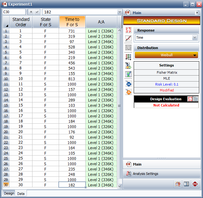
Figure 4: Data entered in Weibull++ for reliability DOE

 

Figure 5 shows the likelihood ratio test results. From the p value in the "Likelihood Ratio Test Table," it can be seen that the life is indeed different for different operation temperatures. The "MLE Information" table displays results for the parameters β, α₀, α₁ and α₂ as Beta, Intercept, A[1] and A[2], respectively.

 

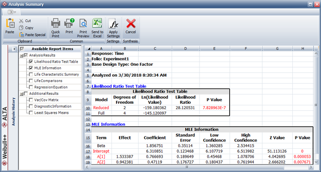
Figure 5: Likelihood ratio test results

 

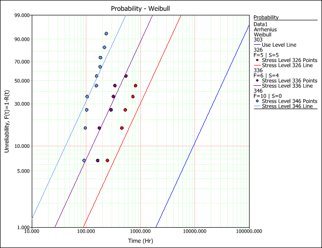
Weibull++ also displays results for pair-wise comparisons of life at different levels. The results are displayed in the "Life Comparisons" table shown in Figure 6. The results indicate that there is a significant difference between life at the operation temperatures of 326 K and 346 K, and also between 336 K and 346 K, but the difference between 326 K and 336 K is not significant. (Figure 7 shows this comparison graphically in a bar chart.) The Z value represents the standardized difference (i.e., the difference divided by the pooled standard error [2]). From Figure 6, it can also be seen that the operation temperature of 326 K gives the largest life characteristic value.

 

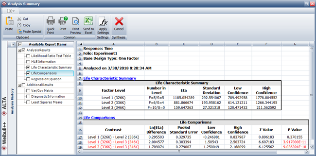
Figure 6: Pair-wise comparisons

 

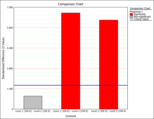
Figure 7: Comparison of the life characteristic

 

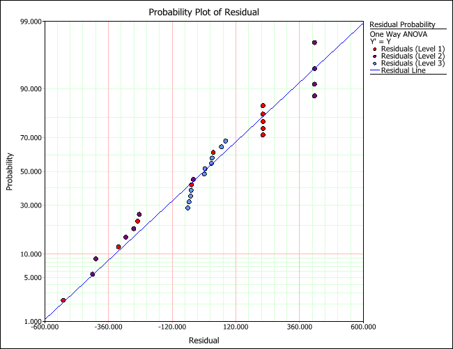
Finally, Figure 8 shows the residual plot for the one factor reliability DOE analysis, which can be compared to Figure 3 to see the applicability of one factor reliability DOE analysis in comparison to one-way ANOVA for this data set.

 

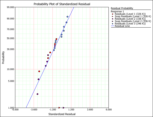
Figure 8: Residual plot for the reliability DOE analysis

 

From the previous discussion, it can be seen that the one factor reliability DOE analysis can be used as an effective substitute for one-way ANOVA to analyze experiments where the response of interest is the life data of a component. The benefits of using the likelihood ratio test can be increased further in cases, such as this one, where the characteristic investigated is a stress that affects the life of the product. In these cases, a predictive model can be obtained using the principles of accelerated life testing analysis, as described next.

 

Accelerated Life Testing Analysis

 

The results of the Weibull++ analysis described in the previous section showed that the investigated characteristic (operation temperature) is a stress that affects the life of the component significantly. However, the DOE analysis is not predictive and cannot be used to make estimates about the failure of the component at different use conditions. So the next step is to obtain a predictive model that quantifies the relationship between the life of the component and the operation temperature and therefore can be used to make such estimations. As described next, this can easily be done by transferring the data to ReliaSoft ALTA software, which includes a selection of life-stress relationships for modeling the life of a product as a function of stress.

 

Predictions Using ALTA

 

The data set from Table 1 can be analyzed in ALTA, as shown in Figure 9. Engineering judgment indicates that the effect of the operating temperature on this component will be well modeled by the Arrhenius life-stress model. Therefore, the equation for the life characteristic can be expressed as follows:

 

(10)

 

where:

 

• η is life characteristic of the data following the Weibull distribution.

• B and C are the parameters of the Arrhenius model.

• Temp is the stress, operation temperature.

 

Figure 9: Data entered and analyzed in ALTA with the Arrhenius-Weibull model

 

ALTA obtains the values of parameters B and C as 13218.16 and 4.9E-15, respectively. Therefore the relationship that models the life of the component as a function of the operation temperature is:

 

(11)

 

Now Eqn. (11) can be used to make predictions regarding the life of the product. Assume that the use temperature of the component is 303K. Figure 10 shows the failure probability plot obtained from ALTA.

 

Figure 10: Weibull probability plot obtained from ALTA

 

To illustrate the use of the prediction model, assume that the analyst wants to predict the B10 life of the component at the use temperature of 303 K. The B10 life is the time by which 10% of the population fails. In other words, the B10 life is the time corresponding to a reliability of 90%. The equation of the reliability of a component that follows the Weibull distribution is:

 

(12)

 

where:

 

• t represents the period of interest or mission time.
• β represents the shape parameter of the Weibull distribution.
• η represents the scale parameter of the Weibull distribution.

 

Substituting the value of η from Eqn. (11), the reliability equation for the electrical component can be written as:

 

 

Entering the values of the parameters obtained from ALTA (as shown in Figure 8), the value of the use temperature (303 K) and the value of the reliability (0.90), the B10 life of the component can be calculated as:

 

 

In ALTA, this value can be obtained directly using the Quick Calculation Pad (QCP), as shown below. Other reliability metrics that may be of interest to analysts can be calculated in a similar manner.

 

 

Conclusion

 

This article demonstrated how one factor reliability DOE analysis can be used to overcome the problems associated with applying one-way ANOVA to life data. The article also presented the use of accelerated life testing data analysis principles to build a reliability prediction model for the cases when the investigated factor is a stress that affects the life of the product.

A future article will explain how reliability DOE can be used as a substitute for traditional DOE techniques involving factorial or fractional factorial designs to investigate a number of factors that are thought to affect product life.

 

References

 

[1] ReliaSoft, "Design for Reliability: Overview of the Process and Application Techniques," Reliability Edge, Volume 8, Issue 2, Tucson, AZ, 2007.

[2] ReliaSoft, Experiment Design and Analysis Reference, ReliaSoft Publishing, Tucson, AZ, 2008.

[3] ReliaSoft, Accelerated Life Testing Reference, ReliaSoft Publishing, Tucson, AZ, 2008.

[4] Kutner, Michael H., Nachtsheim, Christopher J., Neter, John, and Li, William, Applied Linear Statistical Models, McGraw-Hill/Irwin, New York, 2005.

[5] Montgomery, Douglas C., Design and Analysis of Experiments, John Wiley & Sons, Inc., New York, 2001.