Reliability engineering methods are widely applied in design and manufacturing. The process of deploying this collection of tools appropriately is known as Design for Reliability (DFR). Some reliability engineering tools and methods have also been applied in the maintenance sector (i.e., equipment operators) but, in many cases, not as extensively. In this article, we will review the reliability methodologies that are applicable for asset performance management (APM) and propose a process for deploying the appropriate tools at the appropriate stages.
Reliability engineering is a discipline that combines practical experience, maintenance, safety, physics and engineering. Observational data is combined with experience to create models in order to understand the behavior of the equipment, optimize its performance and minimize the life cycle/operational costs. It is important to note that reliability engineering is not simply statistics and it is not always quantitative. Even though quantitative analysis plays a major role in the reliability discipline, many of the available tools and methods are also process-related. It is therefore useful to separate these methods and tools into quantitative and qualitative categories.
In the quantitative category, the typical tools are:
In the qualitative category, the typical tools are:
In this article, we will focus on some of the reliability engineering tools that are the most applicable in asset performance management. This will include a discussion of how and when each method should be deployed in order to maximize effectiveness.
Understanding when, how and where to use the wide variety of available reliability engineering tools will help to achieve the reliability mission of an organization. This is becoming more and more important with the increasing complexity of systems and sophistication of the methods available for determining their reliability. With increasing complexity in all aspects of asset performance management, it becomes a necessity to have a well-defined process for integrating reliability activities. Without such a process, trying to implement all of the different reliability activities involved in asset management can become a chaotic situation in which reliability tools may be deployed too late, randomly or not at all. This can result in the waste of time and resources as well as a situation in which the organization is constantly operating in a reactive mode.
Managers and engineers in the asset management discipline have come to this realization, and a push for a more structured process has been seen in recent years. The circumstances are very similar to what happened with the quality assurance discipline back in the 1980s, which spawned successful processes such as Six Sigma and Design for Six Sigma (DFSS). In more recent years, the same realization occurred in product development with the resulting Design for Reliability (DFR) process. It is therefore natural to look into these successful processes in order to create a process for asset performance management.
The process proposed in this article is based on the Design, Measure, Analyze, Improve and Control (DMAIC) methodology that is widely used in Six Sigma for projects aimed at improving an existing business process. It includes five phases:
To develop the new APM-focused process, we first determined the asset performance management activities within each of these phases. Then we identified the reliability methods and tools that pertain to each activity/phase.
The proposed process can be used as a guide to the sequence of deploying different reliability engineering tools in order to maximize their effectiveness and to ensure high reliability. The process can be adapted and customized based on the specific industry, corporate culture and existing processes. In addition, the sequence of the activities within the APM process will vary based on the nature of the asset and the amount of information available. It is important to note that even though this process is presented in a linear sequence, in reality some activities would be performed in parallel and/or in a loop based on the knowledge gained as a project moves forward. Figure 1 shows a diagram of the proposed process. Each phase in the process is briefly introduced in the following sections.
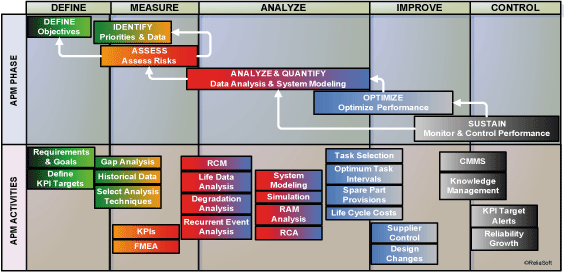
Figure 1: The proposed asset performance management process with applicable reliability engineering tools/methods
The first step of any project is to define its objectives. This phase of the process is very important because it identifies the requirements and goals that will provide a direction for all future phases and activities to be performed. All too often, projects are initiated without a clear direction and without a clear definition of the objectives. This leads to poor project execution. Therefore, it is essential for the organization to do all of the following during the "Define" phase:
The next section provides a brief discussion of the activity that will have the biggest impact on the application of reliability methods/tools in subsequent phases: defining KPIs.
A performance indicator or key performance indicator (KPI) is a measure of performance. Such measures are commonly used to help an organization define and evaluate how successful it is, typically in terms of making progress toward long-term organizational goals. These performance metrics should be monitored in order to assess the present state of the business at any given time, and to assist in prescribing a course of action when improvements are needed.
It is very important that time is spent at the start of a project to define the KPIs that are important to the organization, as well as to review any existing performance indicators to determine their usefulness and how they are obtained from data. Reviewing and understanding the current indicators can also provide a benchmark for judging the success of a project.
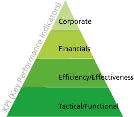
KPIs can be specified by answering the question, "What is really important to different stakeholders?" As such, different levels of performance indicators – corporate, financial, efficiency/effectiveness, tactical/functional – can be specified and aligned to the organization’s business objectives.
Another reason for the critical importance of defining the KPIs at this stage is the impact on future data requirements. In other words, the chosen KPIs will determine what information needs to be captured and analyzed in subsequent phases of the process.
Prior to conducting any type of reliability analysis, it is important to collect all the data required to support the analysis objectives. It is also crucial to determine what kinds of data are available and where the information resides. The types of data available will determine which analyses can be performed so, if sufficient information is not currently available, it may be necessary to identify future steps for obtaining it. Therefore, the typical steps in the "Measure" phase are to perform a reliability gap assessment, then gather the data and select the appropriate analysis techniques.
The purpose of a reliability gap assessment is to identify the shortcomings in achieving the asset performance management objectives so that a reliability program plan can be properly developed. Many companies implement APM tasks without first understanding what drives reliability task selection. The gaps are those issues or shortcomings that, if closed or resolved, would move the company in the direction of achieving its APM targets. In addition, the available data sources can be identified during this activity. If they are inadequate, the analysts may resort to other sources of information. During the gap assessment, answers to the following questions are sought:
Data, and specifically failure time data, are like gold to a reliability engineer. Of course, on the flip side, the more failures that are available to be analyzed, the worse the condition of the asset! In any case, data represent the most important aspect in performing quantitative reliability analyses. It is therefore crucial for data to be collected and categorized appropriately. The data will be used in computing the different KPIs, as well as in performing a variety of reliability calculations.
In addition to failure data, the repair duration is also a very important input in the reliability, availability and maintainability (RAM) model because it determines the equipment availability. Other types of data will also be necessary for a thorough RAM analysis for assets. The following lists provide a summary of the information typically used.
Minimal information required:
Additional information that would improve the analysis if available:
There are multiple sources of data. For example, failure time data can be obtained from maintenance records (work orders, downtime logs, etc.), from the original equipment manufacturer (OEM) reliability specs, or from published generic equipment data.
For existing equipment, historical data can also be used. There may be a great deal of historical data that has been generated over many years. It is necessary to find out where this information resides, and to determine which information can assist in meeting the organization's analysis objectives.
Once the data sources have been identified, the quality and consistency of the data must be evaluated. One of the most common problems for analysis is insufficient quality of the collected data. All too often, even though records are kept, it turns out that the data are not really usable. The most common problems with available data include:
To avoid such problems, it is imperative for the organization to implement corrective actions to ensure that good data collection processes and management are in place.
Finally, assuming that all the relevant information is available, the appropriate simulation and analysis techniques can be selected to estimate the system availability, downtime, production output (a.k.a. throughput), maintenance costs and other metrics of interest.
Depending on the objectives agreed upon during the "Define" phase and the data sources/analysis techniques identified in the "Measure" phase, the next step is to execute the appropriate analysis techniques in order to optimize the performance of the asset. In the following sections, we will briefly highlight the objectives, applications and benefits of some of the most effective reliability-related methodologies that can be used in asset performance management.
RCM analysis provides a structured framework for analyzing the functions and potential failures of physical assets in order to develop a scheduled maintenance plan that will provide an acceptable level of operability, with an acceptable level of risk, in an efficient and cost-effective manner. RCM can be:
A lot has been written about RCM and its benefits. A full discussion of the topic is outside the scope of this article but it is worth mentioning some of the widely accepted benefits, which include:
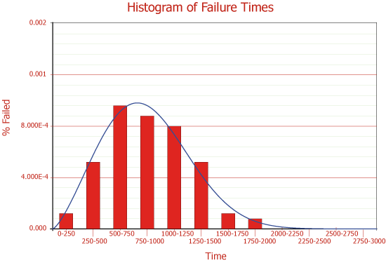
Life data analysis (also called distribution analysis or Weibull analysis) refers to the application of statistical methods in determining the reliability behavior of equipment based on failure time data. Life data analysis utilizes sound statistical methodologies to build probabilistic models from life data (i.e., lifetime distributions, such Weibull, lognormal, etc.). The following graphic shows how a statistical distribution is fitted to failure data.
The probabilistic models are then utilized to compute the reliability, make predictions and determine maintenance policies and maintenance task intervals. These models should be applied at the lowest replaceable unit (LRU) level. Some of the applications for this type of analysis include:
Another way to calculate reliability metrics involves a type of analysis known as degradation analysis. Many failure mechanisms can be directly linked to the degradation of part of the product. Assuming that this type of information is captured (e.g., condition based maintenance – CBM – data), degradation analysis allows the engineer to extrapolate to an assumed failure time based on the measurements of degradation over time. This analysis essentially determines the P-F curve that is often discussed by RCM practitioners (i.e., the period from when it is possible to start to recognize a potential failure, P, until it becomes an actual failure, F). The degradation analysis results can be used to:
RDA is different than "traditional" life data analysis (distribution analysis) because RDA builds a model at the equipment/subsystem level rather than the component/part level. Furthermore, whereas life data analysis uses time-to-failure data (in which each failure represents an independent event), the data utilized in RDA are the cumulative operating time and the cumulative number of failure events. Therefore, while life data analysis is used to estimate the reliability of non-repairable components, RDA models are applied to data from repairable systems in order to track the behavior of the number of events over time and understand the effectiveness of repairs. The most commonly used models for analyzing recurrent event data are the non-homogeneous Poisson process (NHPP) and the general renewal process (GRP).
A reliability, availability and maintainability (RAM) analysis typically starts from the creation of a diagram that represents the overall system/process and the corresponding major subsystems. This diagram is known as a reliability block diagram (RBD). The next step is to expand the major subsystems into subsubsystems and keep repeating until you reach the level where reliability information is available (ideally at the LRU level). The analysis will be based on the failure and repair duration properties for the items in the diagram. The failure properties (i.e., reliability) determine the frequency of occurrence of failure of each LRU; the repair durations determine the downtime. The effect of the failure on the overall system is determined based on the configuration of the block diagram. The effect could be that the entire system fails or it could be a percent reduction in the total output (throughput) of the system.
To perform a complete RAM analysis, the following information is required:
The results of such an analysis may include:
Having the system RBD model will also help later in the "Improve" phase to perform what-if analyses and investigate the effect of any proposed changes/improvements.
RCA is a method to logically analyze failure events, identify all the causes (physical, human and primary) and define corrective actions to prevent their recurrence. It is a critical activity in understanding failures and being able to determine corrective actions. Without a formal RCA procedure, the wrong remedies might be frequently implemented.
The main objective of an APM process is to drive improvements, thus the "Improve" phase represents the most critical step of the process. During this phase, the objective is to identify the improvements that can increase the performance of the asset and optimize it, including:
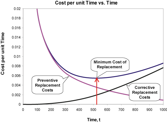
As an example, the following section provides a brief overview of one of the most commonly used reliability tools that can be employed in this phase: calculating the optimum preventive maintenance (PM) interval.
Engineers can use the following equation to find the optimum interval for a preventive maintenance action. The equation is solved for the time, t, that results in the least possible cost per unit of time.
![]()
where:
This calculation is also demonstrated graphically in the following picture.
Every time the APM process is initiated, it is imperative to execute activities that can sustain the achieved results. As such, certain activities to monitor and control the performance need to be applied during the "Control" phase, including:
Another critical function in this phase is sustaining the knowledge acquired by all previous activities, as well as retaining the analyses that have led to a particular action or change. Failing to retain this knowledge can lead to "reinventing the wheel" down the road, as well as the risk of repeating past mistakes. Different activities (including analysis, action plans and decisions) should be recorded properly and stored in a location where other professionals involved in the asset’s management can access the information in the future.
In this article, we reviewed the role of reliability engineering methodologies in asset performance management, and we proposed a flexible APM process for deploying different reliability tools and methods where they can be most effective. The proposed process is general enough to be easily adopted by different industries and can be used in conjunction with current reliability practices.
[1] T. Wireman, Developing Performance Indicators for Managing Maintenance, 2nd ed., New York, NY: Industrial Press, Inc., 2005.
[2] ReliaSoft, Life Data Analysis Reference, Tucson, AZ: ReliaSoft Publishing, 2005.
[3] ReliaSoft, System Reliability Reference, Tucson, AZ: ReliaSoft Publishing, 2007.
[4] A. Mettas and W. Zhao, "Modeling and Analysis of Repairable Systems with General Repair," in the 2005 Proceedings of the Annual Reliability and Maintainability Symposium, 2005.

This will bring together HBM, Brüel & Kjær, nCode, ReliaSoft, and Discom brands, helping you innovate faster for a cleaner, healthier, and more productive world.
This will bring together HBM, Brüel & Kjær, nCode, ReliaSoft, and Discom brands, helping you innovate faster for a cleaner, healthier, and more productive world.
This will bring together HBM, Brüel & Kjær, nCode, ReliaSoft, and Discom brands, helping you innovate faster for a cleaner, healthier, and more productive world.
This will bring together HBM, Brüel & Kjær, nCode, ReliaSoft, and Discom brands, helping you innovate faster for a cleaner, healthier, and more productive world.
This will bring together HBM, Brüel & Kjær, nCode, ReliaSoft, and Discom brands, helping you innovate faster for a cleaner, healthier, and more productive world.
This will bring together HBM, Brüel & Kjær, nCode, ReliaSoft, MicroStrain and Discom brands, helping you innovate faster for a cleaner, healthier, and more productive world.