Degradation Data Analysis

Modeling the Destructive Degradation Analysis

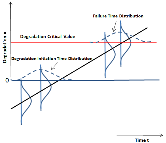
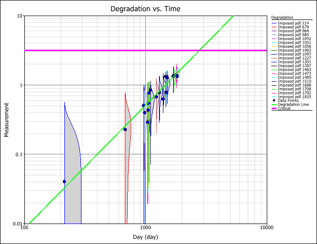
A level of degradation or performance at which a failure is said to have occurred should be defined when performing degradation analysis. To obtain time-to-failure data, basic mathematical models can be utilized to extrapolate the measurements over time to the point where the failure is said to occur. These extrapolated failure times can be easily analyzed in the same manner as conventional time-to-failure data.

However, having only one degradation measurement for each item tested, it is impossible to build a degradation model for each individual item and use the model to predict failure time. Therefore, a statistical distribution is needed to represent the variability in the measurement at a given time. This method is called the random process modeling method. In this method, the degradation value is assumed to be a random variable that follows a certain distribution at a given time. In the ReliaSoft Weibull++ destructive degradation analysis folio, any of the following distributions can be used to define the variability in the degradation measurements: Weibull, exponential, normal, lognormal, or Gumbel.

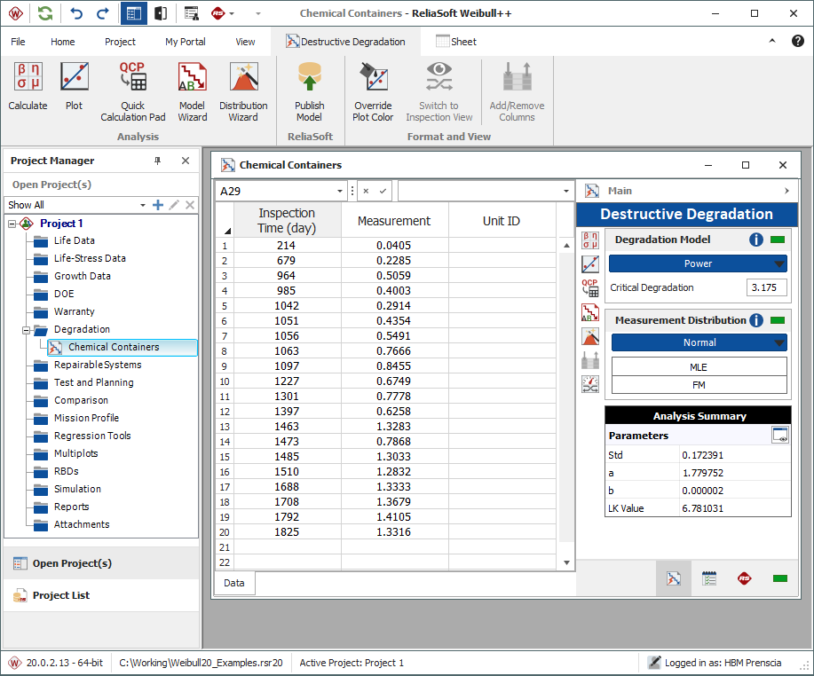
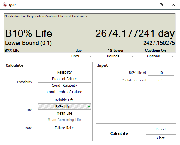
For example, we can assume that the corrosion in a chemical container follows a Weibull distribution at any given time. Subsequently, the scale parameter (η) will decrease with time as the container corrodes over time, while the shape parameter (β) will stay constant since the process of corroding will not change.

The random process modeling method requires that the scale parameters are defined over the entire domain from –∞ to ∞. However, eta (η) for the Weibull distribution and Mean-Time-To-Failure (MTTF) for the exponential distribution are always greater than zero. Thus, natural logarithms of these parameters are used in the random process modeling method. For each distribution the parameters are defined as:

• Weibull: ln(η) is set as a function of time while β remains constant.
• Exponential: ln(MTTF) is set as a function of time.
• Normal: μ is set as a function of time while σ remains constant.
• Lognormal: μ' is set as a function of time while σ' remains constant.
• Gumbel: μ is set as a function of time while σ remains constant.
   

Once the distribution is selected, the change of the scale parameter with time needs to be defined by a degradation model. Several models are good candidates and used in Weibull++:

• Linear: μ(t) = b + a × t
• Exponential: μ(t) = b × exp^(a × t)
• Power: μ(t) = b × t ^a
• Logarithm: μ(t) = a × ln(t) + b
• Lloyd-Lipow: μ(t) = a − (b/t)
   

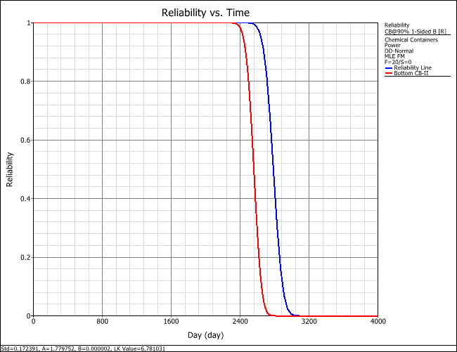
After the distribution and degradation models are chosen and their parameters are defined, the parameters are then calculated using Maximum Likelihood Estimation (MLE).

Previously, we assumed that the corrosion in a chemical container follows a Weibull distribution at any given time. Hence, the unreliability at time t can be derived as:

The scale parameter function can be any commonly used degradation function as was described earlier (i.e., linear, logarithm, power, etc.). Recall that the eta (η) for the Weibull distribution and Mean-Time-To-Failure (MTTF) for the exponential distribution cannot be defined in the negative domain. Therefore, natural logarithms of these parameters are used. We will assume that the scale parameter changes linearly in this example and can be formulized as:

The parameters (a, b and β) are then calculated using Maximum Likelihood Estimation (MLE).

The following plot illustrates the relationship between the distribution of the degradation measurement and the distribution of failure times.

Example

Assume that you are a reliability engineer working at a chemical storage container manufacturing company. You are responsible for testing the reliability of the carbon steel containers that are used for storing 98% concentrated sulfuric acid with a specific gravity of 1.8437 g/cm3 at 60 °F.

You already know that sulfuric acid reacts with the iron in the shell to form a ferrous sulfate product and hydrogen. Ferrous sulfate protects the container’s wet surfaces from the acid. However, this protective layer may deteriorate due to many conditions such as agitation, dilution of the acid, high temperatures, etc. The steel will corrode without this protective layer, reducing the thickness of the container walls.

As the reliability engineer, you want to know how long it would take for the storage containers to fail while storing sulfuric acid. The failure criterion for the storage containers (design corrosion allowance) is defined as the time when the wall thickness wears down by 1/8 inches (3.175 mm). You run a test on 20 storage containers with sulfuric acid and collect the corrosion data over a 5 year period, as provided in the table below. You only have a single measurement for each container since you need to destroy the container to get the most accurate measurement. You use destructive degradation analysis to analyze the data.

You enter the data in a Weibull++ destructive degradation folio and analyze the data using the Power model for the degradation model and the Normal distribution for the failure data. The results show that standard deviation = 0.1724, a = 1.7798 and b = 2 × 10⁶.

The following plot shows the change of the wear distribution with time. The horizontal line represents the critical degradation level (the time when the wall thickness reaches 3.175 mm).

The following reliability vs. time plot shows the probability that the component wear will be less than 3.175 mm at different times of operation (blue line). The lower 1-sided 90% confidence bound is shown on the plot as well (red line).

The B10 life of the containers while storing sulfuric acid (i.e., the time by which 10% of containers will exhibit a wear greater than 3.175 mm) is approximately 2,674 days (7.33 years). The lower 1-sided 90% bound on the B10 life is 2,427 days (6.65 years), as shown next.

References

1. Guo, H., Liao, H. "Practical Approaches for Reliability Evaluation Using Degradation Data," Annual Reliability and Maintainability Symposium, January 2015.
2. ReliaSoft Corporation. 2015. "Degradation Data Analysis," http://ReliaWiki.org/index.php/Degradation_Data_Analysis
3. Inyo Process. 2015. "Specific Gravity and Weights of Sulfuric Acid," PDF file,http://www.inyoprocess.com/images/chem_appl/sulfuric acid properties.pdf
4. Office of Environment, Health and Safety of the University of California, Berkley. 2015. "Safe Storage of Hazardous Chemicals," PDF file, http://ehs.berkeley.edu/sites/default/files/lines-of-services/hazardous-materials/chemicalstoragebooklet.pdf