登録完了

1. Equivalent circuit diagram of the transformer

Figure 1 shows the operating principle of a transformer with two windings that are magnetically connected with a ferrite core. Due to the high permeability of the ferrite core in comparison to the air, the flux is directed through it. Nonetheless, slight leakage fluxes  and  do occur. Resistances  and simulate the ohmic part of the windings. To describe the operating behavior of the transformer, an equivalent circuit diagram is derived from this model as shown in Figure 2. This diagram shows the transmission ratio between the primary and secondary side for an ideal transformer. The other effects that occur are represented by passive components. The magnetic fluxes are described by the leakage inductances  and, and also by the main inductance. The resistor is connected in parallel to the main inductance and serves to simulate the iron losses in the core material. These consist of eddy current losses and hysteresis losses.

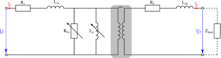
Eddy current losses arise due to a current flow in the ferrite core which is caused by induced voltages. In accordance with Lenz's law, this current opposes the change that caused it. To minimize the current flow, the ferrite core is made up of plates that are isolated from each other. The hysteresis losses are caused by the periodic remagnetization of the ferrite core, since energy is required to align the molecular magnets in the iron (Weiss domains). Since both the main inductance L_µ and the iron loss resistance R_Fe are dependent on the core material with non-linear permeability µ_Fe, both follow a non-linear course. R_K = R₁ + R₂ ü²     (1)

L_K = L_1σ + L_2σ ü²   (2) The leakage inductances may be considered as linear, since their field lines run primarily through the air, which exhibits constant permeability. For further considerations the equivalent circuit diagram from Figure 2 is simplified still further (Figure 3). The voltage drop on R₁ and L_1σ is negligibly small in comparison to the voltage drop due to the iron loss resistance R_Fe and the main inductance L_µ in normal operation. This makes it possible to contact the iron loss resistance R_Fe and main inductance L_µ directly with the input terminals. [1] In equations (1) and (2) the ohmic resistance R₂ and the leakage inductance L_2σ of the secondary side are converted to the primary side and combined to form R_K and L_K. The measurements and calculations performed below refer to the equivalent circuit diagram simplified in this manner. Quantities I'₂, U'₂ and Z' _load have been converted from the secondary side to the primary side taking into consideration the transmission ratio.

2. Measurements in no-load

The values of the iron loss resistance R_Fe and main inductance L_µ can be determined by a no-load test as shown in Figure 4. Since these values exhibit non-linear behavior, the unloaded transformer is supplied with a variable transformer as a sinusoidal voltage source with variable amplitude. This makes it possible to approach and measure different load points with differently linked magnetic flux Ψ. The magnetic flux is calculated from the applied voltage as follows: Ψ = ∫▒ u ̂⋅ sin(2πft)dt     (3)
Ψ = -u ̂/2πf ⋅ cos(2πft)    (4) The metrologically acquired quantities are the primary voltage u₁ (t), primary current i₁ (t) and secondary voltage u₂ (t). To determine the iron loss resistance R_Fe and main inductance L_µ, first the root mean square value of the primary voltage U₁, the primary-side active power P₁ and the reactive power Q₁ are determined. The calculations are performed on a cyclical basis. The component values and transmission ratio ü can be calculated with formulas (5) (6) and (7). R_Fe = U₁²/P₁                        (5)

L_µ = 1/(2 π f) ⋅ (U₁²/Q₁)    (6)

ü = U₁/U₂                             (7) As can be seen in Figure 5, the component values are not constant due to dependence on the magnetic flux. The calculated component values are an average over a sine wave.

The measured values are examined over the course of time to allow for further examination. The distortion of the current over time (red curve) is clearly seen in Figure 6. The core material runs into saturation. The correlation between the flux density B and the magnetic field strength H is illustrated most vividly by the hysteresis curve. If the core geometry is known, the flux density and field strength can be determined from the measured quantities with: B = Ψ/A_Fe        (8) H = I/l_Fe          (9) Due to the unknown core geometry of the test specimen measured here, the hysteresis curve is realized in Figure 7 as a ΨI characteristic curve. The new curve and a number of load points are also shown in Figure 8. The new curve is determined by approaching different load points in which the linked flux and current are acquired in the voltage zero crossing. It is produced when a field strength is first applied to an unmagnetized core and is the characteristic curve of the main inductance L_µ. The flux density increases slowly at first. As the field strength increases, the flux density increases faster and faster until the core goes into saturation and the flux density hardly rises at all. Now if the field strength is reduced, the flux density does not return on the new curve. Instead it follows the hysteresis curve. When the field strength is equal to zero a residual magnetism remains, referred to as remanence. The field strength required to eliminate the residual magnetism is called the coercive field strength. [2]

Another method for determining the expected iron losses is the Steinmetz formula (10). P_Fe = k ⋅ f^a ⋅ Ψ^b           (10) The Steinmetz formula is based on the fact that the surface enclosed by the hysteresis curve is equal to the iron losses. The precondition for applying the Steinmetz formula is a sinusoidal input voltage. The iron losses for differently linked flux calculated from the measured values can be used to determine the unknown coefficients a and b from formula (10) by curve fitting (Figure 9). The curve produced in this manner can then be used to estimate iron losses for other load points in advance.

3. Measurements in the short circuit

In the short-circuit test the secondary side is short-circuited by a low-ohm impedance Z_load (Figure 11). The current is set to the nominal (rated) current by a variable transformer.

The current through the main inductance and iron loss resistance is negligible in this operating state. The quantities acquired metrologically are the primary voltage u₁ (t), primary current i₁ (t), secondary current i₂ (t) and the voltage u₂ (t) over the load. First the voltage drop is calculated with R_K and L_K. u_K (t) = u₁ (t) - ((u₂ (t))/ü)         (11) Then u_K (t) and i'₂ (t) can be used to calculate the power transformed on R_K and L_K and the component values can be calculated. R_K = P_K / I'_2²     (12)
L_K = 1/2π f ⋅ (Q_K / I'₂²)    (13)