웨이불++ 신뢰성 향상 - 간단한 MTBF 결정

A new helicopter system is under development. System failure data are collected on five helicopters during the final test phase. The total number of flight hours is 500, accrued over a period of 12 weeks. The 500 flight hours are partitioned into six intervals, each covering a two-week period. Every two weeks, each helicopter undergoes a thorough inspection to uncover any failures that may have occurred since the last inspection. Therefore, although the actual failure times are unknown, the analysts have the cumulative total number of flight hours and the cumulative total number of failures for the five helicopters for each two-week period.

Interval #	Interval Length in Flight Hours	Failures in Interval
1	0 - 62	12
2	63-100	6
3	101 - 187	15
4	188 - 210	3
5	211 - 350	18
6	351 - 500	16

Analysis and discussion

 

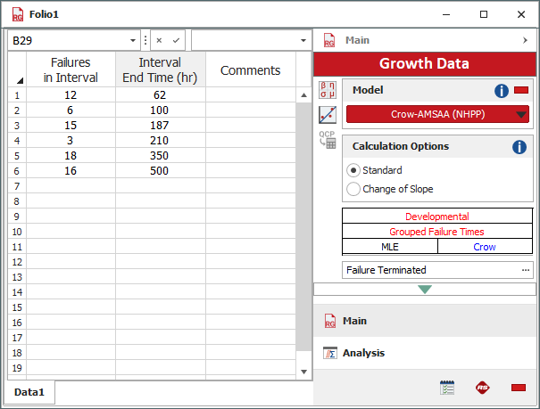
A standard folio data sheet configured for grouped failure times data type is created by selecting Times-to-Failure Data > Grouped Failure Times on the first page of the Project Item Wizard window, as shown next.

Figure 1: Selecting the data type and units of measurement for the new folio

The data set is then entered and the Crow-AMSAA (NHPP) model is selected for analysis, as shown next.

Figure 2: Data set entered in the standard folio

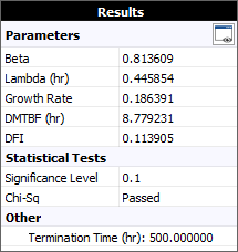
After analyzing the data, the results summary shows that the demonstrated failure intensity (DFI) value at the end of the 28 hours of testing is 4.4947.

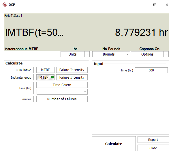
This can also be seen by using the Quick Calculation Pad (QCP). Since the test ended at 28 days, the DFI is equal to the instantaneous FI at 28 days, as shown next.

Figure 4: Quick calculation showing the DFI (i.e., failure intensity at the end of the test)

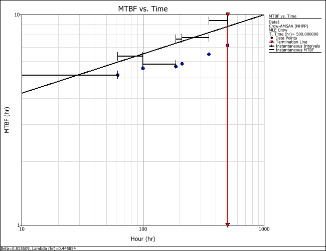
A plot of the MTBF vs. time is shown next. The plot shows the mean time between failures plotted against time. The horizontal lines represent the instantaneous MTBF over the marked interval. The points represent actual failures in the data set.

Figure 5: MTBF vs. time plot showing both instantaneous and cumulative MTBF

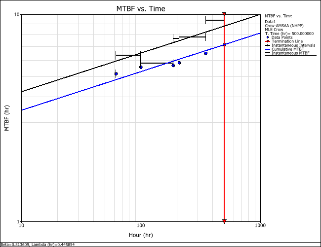
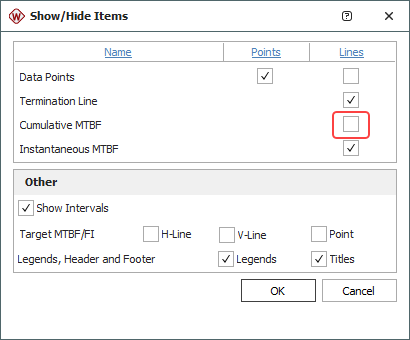
The cumulative MTBF line is then removed by right-clicking the plot.

Figure 6: Show/Hide Items window with cleared option for cumulative MTBF line

The plot now looks like this.

Figure 7: MTBF vs. time plot showing only instantaneous MTBF