내구성 테스트, 신뢰성 및 장애 모드 비교

Let’s assume you are an engineer tasked with validating the durability of a structural part that is susceptible to fatigue cracking. Proving ground tests are often used to assess component durability, but unfortunately they can be costly and time consuming. A laboratory durability test is desirable due to reduced variability, cost, and time but you then face the challenge of moving the durability test into the lab while replicating the same failure behavior. 

If fatigue is the failure mode, fatigue methodologies like Stress-Life (SN) can be used to create an equivalent fatigue damage test specification. This way, the complicated loading seen on the proving ground can be converted into simplified test lab loading that produces the same amount of fatigue damage. Once a relative damage relationship has been determined, the lab test can be run and results from the proving ground and lab can be compared statistically with reliability methods to assess the failure behavior and answer these critical questions:  

• Are these failure modes the same? 
• Is the lab test representative of real product usage?

Durability testing, reliability, and failure mode comparison

Let’s assume you are an engineer tasked with validating the durability of a structural part that is susceptible to fatigue cracking. Proving ground tests are often used to assess component durability, but unfortunately they can be costly and time consuming. A laboratory durability test is desirable due to reduced variability, cost, and time but you then face the challenge of moving the durability test into the lab while replicating the same failure behavior. 

If fatigue is the failure mode, fatigue methodologies like Stress-Life (SN) can be used to create an equivalent fatigue damage test specification. This way, the complicated loading seen on the proving ground can be converted into simplified test lab loading that produces the same amount of fatigue damage. Once a relative damage relationship has been determined, the lab test can be run and results from the proving ground and lab can be compared statistically with reliability methods to assess the failure behavior and answer these critical questions:  

• Are these failure modes the same? 
• Is the lab test representative of real product usage?

This process can be performed in three general steps:

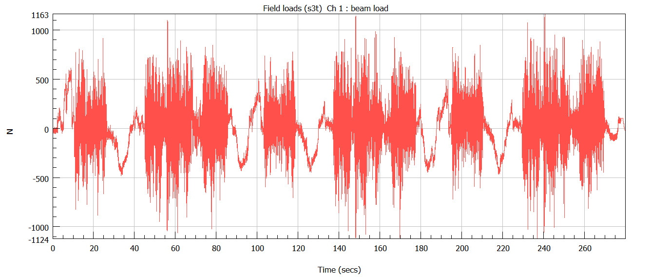
Step 1: Assessing fatigue cyclic content

The structural loading this part experiences in the proving ground has been measured and is shown above. This measured data contains a broad spectrum of cycles – from small to large – all of which contribute to the overall fatigue damage.  

The most common method of quantifying cyclic content for fatigue calculations is rainflow cycle counting.  Results are shown below.

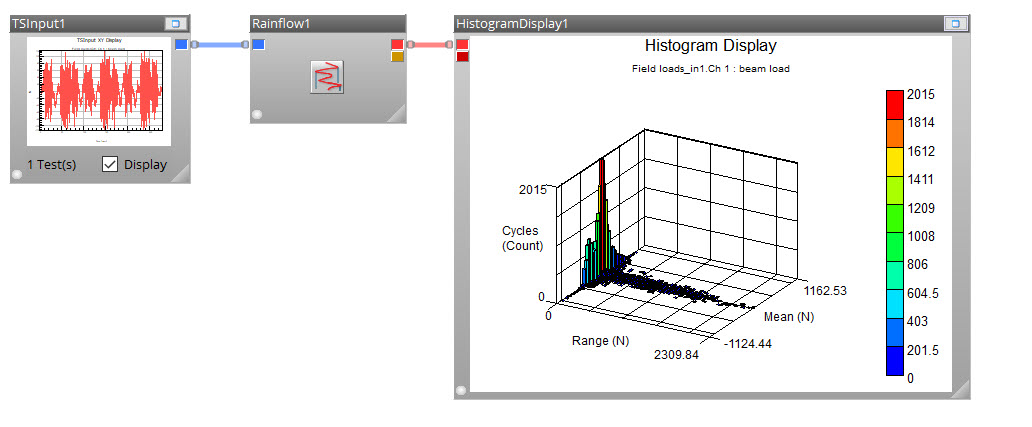
Once this spectrum of cycles is counted, a cycle size can be chosen to be replicated in the simplified lab test. The cycle size should not be larger than the largest cycle observed in the measured loading or else the failure mode may be changed. Additionally, a very small cycle size might require a very lengthy test in order to replicate equivalent fatigue damage. Therefore, a balance must be made to select a cycle size that is large enough for the lab test to complete within a target duration, yet not too large.

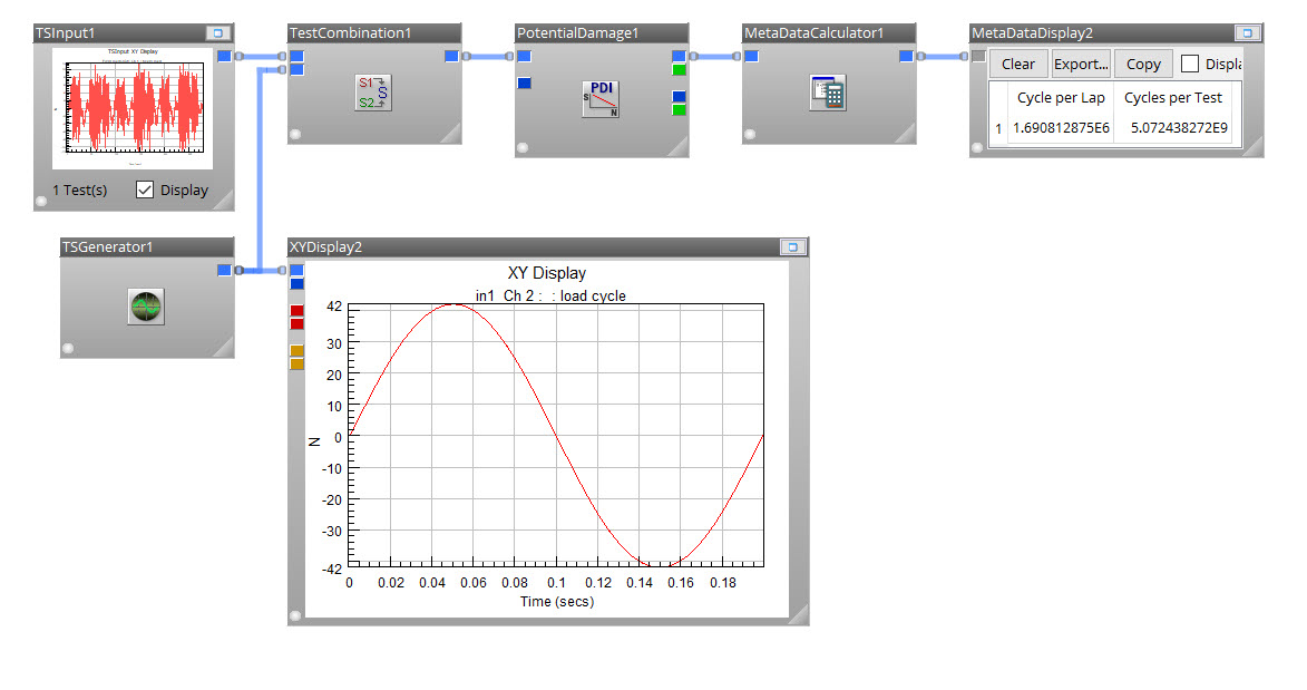
Step 2: Calculating equivalent damage loading

The final step is to compare the failure behavior from the track test and lab test(s). It is possible to perform forensics on the broken faces of a failed part to assess the failure mode. Alternatively, the life data results from each population of failed parts can be modelled statistically and compared. While several statistical models could be used, Weibull is often selected due to its flexibility. The parameters β and η can describe the failure behavior and time to failure respectively. When using a level of confidence, these parameters can then be described as ranges.

Step 3: Failure mode comparison

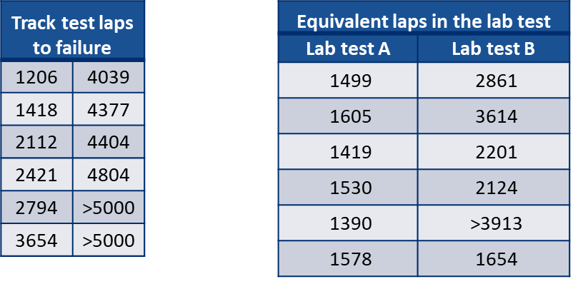
Suppose you followed the steps above and create two possible test loading specs:

• Lab test A: A large cycle repeated 50,000 times
• Lab test B: A small cycle repeated 200,000 repeats

Test A has clear benefits in that it will take less time to get results! But maybe you want to know which option is a better durability test. 

You run the product validation test using both newly-created equivalent damage lab loadings, failing 6 samples in each test. Fatigue damage calculations allow the lab failure times to be correlated back to equivalent proving ground laps. Previous testing on the proving ground also returned 6 failures.

The final step is to compare the failure behavior from the proving ground and lab test(s). It is common to perform forensics on the broken faces of broken parts to assess the failure mode – with the assumption that similar failure surfaces implies similar failure modes.

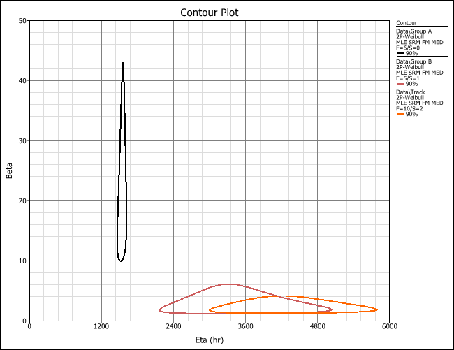
Statistics can also aid this comparison. The life data results from each population of failed parts can be statistically modelled and compared. While several statistical models could be used, the Weibull distribution is often selected due to its flexibility. Weibull parameters β and η can describe the failure behavior and time to failure, respectively. These values can be calculated for each set of failure data and then compared to assess similarities or differences. Further, confidence bounds can be introduced and these parameters can then be described as ranges.

Once each population is modeled, β and η at a specified level of confidence can be compared. Visually, the easiest comparison method is on a contour plot. Separation between contours signifies populations are statistically different at the specified level of confidence.

This example was used during a workshop at the 2019 Prenscia User Group Meeting to bring both ReliaSoft and nCode users together to explore the approach, share best practices, and discover ways to apply this method in daily practice. We have found that this approach works well for creating lab test from proving grounds with equivalent damage. We are confident that if you need to create a lab test specification, this method will allow you to reduce test time and cost while assessing failure mode behavior. 

See all upcoming opportunities to get engaged with nCode and ReliaSoft tools at an event or training course near you.