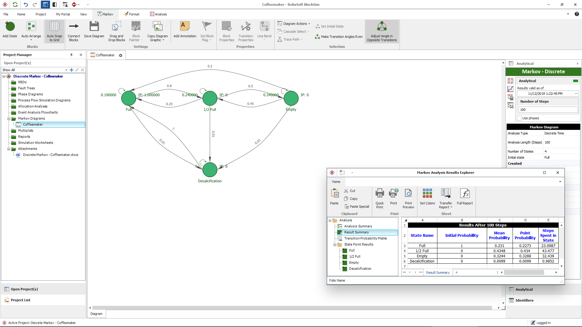
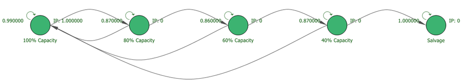
With BlockSim, we will demonstrate an initial estimation analysis on the life cycle of a complex drilling system that starts off as brand new (100% initial probability in the full capacity state). The system has a probability to degrade into various states of capacity with time and can eventually enter a salvage state. There is also a probability of being returned to the as-good-as-new condition from each degraded state, except from the salvage state. The salvage state is considered to be a "sink," a state from which there are no transitions to any other state and therefore we have zero probability of leaving. We want to determine, on average, what percent of the time will be spent in each state over a 10-year period. To perform this type of analysis, we will use a discrete Markov diagram. Our initial setup looks like this:
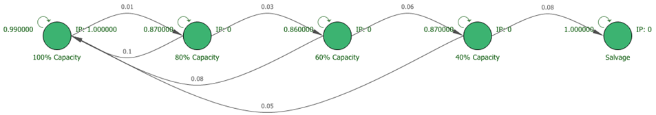
We estimate the following probabilities per month to move between states:
Based on these percentages, the final diagram that is ready for analysis looks like this:
Since our estimated probabilities are on a month scale, we will take each step of the analysis to be the equivalent of one month. This means that we will run our calculation for 120 steps. After we calculate the diagram, we can see that the transition probability matrix between the states looks like this (which we can easily use to verify our inputs):
| Full Diagram | |||||
|---|---|---|---|---|---|
| FROM -> TO | 100% capacity | 80% capacity | 60% capacity | 40% capacity | Salvage |
| 100% capacity | 0.99 | 0.01 | 0 | 0 | 0 |
| 80% capacity | 0.1 | 0.87 | 0.03 | 0 | 0 |
| 60% capacity | 0.08 | 0 | 0.86 | 0.06 | 0 |
| 40% capacity | 0.05 | 0 | 0 | 0.87 | 0.08 |
| Salvage | 0 | 0 | 0 | 0 | 1 |
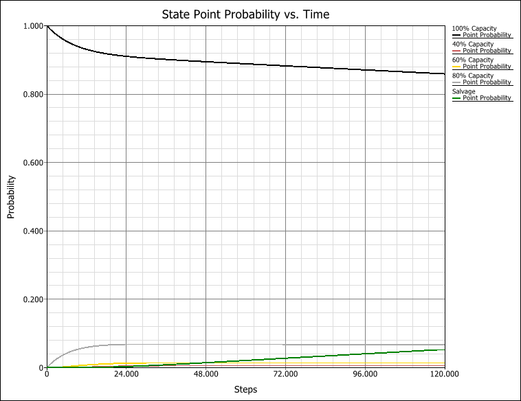
In this case study example, because we have a "sink" state, we do not reach steady state, where all the probabilities have reached a constant value, but rather a pseudo-steady state where the probabilities are changing at a roughly constant rate.
Afterwards, we can check the results summary to determine the mean probabilities in each state and the point probabilities after 120 steps (10 years).
| Results After 120 Steps | ||||
|---|---|---|---|---|
| State name | Initial probability | Mean probability | Point probability | Steps spent in state |
| 100% capacity | 1 | 0.894127 | 0.859252 | 107.295203 |
| 80% capacity | 0 | 0.064845 | 0.066382 | 7.781451 |
| 60% capacity | 0 | 0.013046 | 0.014282 | 1.565469 |
| 40% capacity | 0 | 0.005597 | 0.00662 | 0.671615 |
| Salvage | 0 | 0.022386 | 0.053464 | 2.686261 |
From the results we can conclude that the majority of the time (89.4%) our system should be running at 100% capacity and that after the 10-year period there is about a 5.3% chance that the system will degrade to a point from which it cannot be restored (the salvage state).